Beilinson's Resolution of the Diagonal
April 2025
Plan
The goal of this talk is to understand a certain 2 page paper of Beilinson entitled “Coherent Sheaves on \(\mathbb{P}^n\) and Problems of Linear Algebra”, as well as some of its implications. Here’s the plan:
Write down “Beilinson’s Resolution of the Diagonal” (a certain locally free resolution of \(\mathcal{O}_{\Delta} \in \mathrm{Coh}(\mathbb{P}^n\times \mathbb{P}^n)\))
Use this resolution to see how \(\mathcal{O}(-n),\dots,\mathcal{O}\) (and its “dual”) form a “basis” for the derived category \(D^b(\mathbb{P}^n)\) (in the sense that they form a full strong exceptional collection).
Sketch a derived equivalence between \(\mathrm{Coh}(\mathbb{P}^n)\) and certain quiver representations (a way of equipping a certain directed graph with vector spaces and linear maps).
These notes mostly come from Calabrese’s On a Theorem by Beilinson, with some other pieces from Skowronski, Simson, Assem’s Elements of the Representation Theory of Associative Algebras: Volume 1: Techniques of Representation Theory.
Beilinson’s Resolution of the Diagonal
Setup
Write \(\mathbb{P}=\mathbb{P}^n\), and denote projections from \(\mathbb{P}\times \mathbb{P}\) to its factors as follows.

Let \(\Delta: \mathbb{P}\to \mathbb{P}\times \mathbb{P}\) be the diagonal map. Our goal is to write a locally free resolution of \(\mathcal{O}_\Delta :=\Delta_* \mathcal{O}_\mathbb{P}\) consisting of certain box products. We explain our strategy here.
We have vector bundles \(\mathcal{O}_\mathbb{P}^{n+1}\) and \((\mathcal{O}_\mathbb{P}^{n+1})^\vee\), and we can form their box product together with an “evaluation” map \[\mathcal{O}_\mathbb{P}^{n+1} \boxtimes (\mathcal{O}_\mathbb{P}^{n+1})^\vee = q^* \mathcal{O}_\mathbb{P}^{n+1} \otimes p^* (\mathcal{O}_\mathbb{P}^{n+1})^\vee \cong \mathcal{O}_{\mathbb{P}\times\mathbb{P}}^{n+1} \otimes (\mathcal{O}_{\mathbb{P}\times\mathbb{P}}^{n+1})^\vee \xrightarrow{\mathrm{eval}} \mathcal{O}_{\mathbb{P}\times \mathbb{P}}\] by sending \[s \otimes \phi \longmapsto \phi(s).\] Defined as is, \(\mathrm{eval}\) is surjective, so the cokernel is 0. However, we will pick bundles \[\mathcal{O}_\mathbb{P}(-1) \hookrightarrow \mathcal{O}_\mathbb{P}^{n+1}, \qquad \Omega_\mathbb{P}(1) \hookrightarrow (\mathcal{O}_\mathbb{P})^{n+1}\] so that the image of restricted \(\mathrm{eval}\) is instead the ideal sheaf of \(\Delta\), so that the cokernel is \(\mathcal{O}_{\Delta}\) as desired.
Denoting \[\mathcal{E}= \mathcal{O}_\mathbb{P}(-1) \boxtimes \Omega_\mathbb{P}(1),\] we will be able to start our resolution of \(\mathcal{O}_\Delta\) by \[\mathcal{E}\to \mathcal{O}_{\mathbb{P}\times \mathbb{P}} \to \mathcal{O}_\Delta \to 0.\] We will then be able to finish up the resolution using the Koszul complex, as in the following proposition.
Proposition. Let \(\mathcal{E}\) be a locally free sheaf of rank \(r\) on a scheme \(X\), and \(s\in \Gamma(\mathcal{E}^\vee)\) a global section of the dual. Then, there is a complex called the Koszul complex \[0 \to \bigwedge^r \mathcal{E}\to \cdots \to \bigwedge^1 \mathcal{E}\to \bigwedge^0 \mathcal{E}\to \mathcal{O}_{V(s)} \to 0,\] and if \(X\) is locally Cohen-Macaulay and \(\mathrm{codim}V(s) = r\), then it is exact.
Proof. We can identify \(\bigwedge^i \mathcal{E}\) as a subsheaf of a tensor product, (as in the differential geometry-esque style of wedge product as alternating functionals on the dual) \[\bigwedge^i \mathcal{E}\hookrightarrow \bigwedge^{i-1} \mathcal{E}\otimes \mathcal{E},\] by hitting the following morphism of presheaves with sheafification \[e_1 \wedge \cdots \wedge e_i \longmapsto \sum_{\ell=1}^i (-1)^\ell e_1 \wedge \cdots \wedge \hat{e_\ell} \wedge \cdots \wedge e_i \otimes e_\ell.\] Then, we have a morphism \[\bigwedge^{i-1} \mathcal{E}\otimes \mathcal{E}\to \bigwedge^{i-1} \mathcal{E}\otimes \mathcal{O}_X \cong \bigwedge^{i-1} \mathcal{E}\] from \(\mathcal{E}\xrightarrow{s} \mathcal{O}_X\). Now, the composition of these morphisms is \[\bigwedge^i \mathcal{E}\to \bigwedge^{i-1} \mathcal{E}\] which is referred to as contraction with \(s\).
Now, on stalks, choosing an identification \(\mathcal{E}_x \cong \mathcal{O}_{X,x}^r\), our morphism \(s: \mathcal{E}_x \to \mathcal{O}_{X,x}\) gets identified with a morphism \(\mathcal{O}_{X,x}^r \to \mathcal{O}_{X,x}\) defined by sending the basis \(e_1,\dots,e_r\) to germs \(f_1,\dots,f_r\). Then, under this identification, the complex we defined is exactly the usual Koszul complex \(K(f_1,\dots,f_r)\) on the local ring \(\mathcal{O}_{X,x}\).
So, this tells us in particular that our sequence of morphisms between sheaves \(\bigwedge^i \mathcal{E}\) is a complex. We can also say something about exactness. Assume now that \(X\) is locally Cohen-Macaulay and \(\mathrm{codim}V(s)=r\), and let \(x\in X\) be a closed point. Then, we want to know that \(f_1,\dots,f_r\) is a regular sequence, but this follows from (Bruns and Herzog 1998, Theorem 2.1.2), since \(\dim \mathcal{O}_{X,x}/(f_1,\dots,f_r) = r\) by our codimension assumption. So, our complex is exact when we take stalks at any closed point, so our complex is exact. ◻
Tautological Bundle
Consider this copy of \(\mathbb{P}\) as having homogeneous coordinates \(x_0,\dots,x_n\).
We recall that \(\mathcal{O}_\mathbb{P}(-1)\) is the tautological line bundle, i.e., it naturally can be considered as a subsheaf of \(\mathcal{O}_\mathbb{P}^{n+1}\) (which we think of as having basis vectors \(e_0,\dots,e_n\)) with a fiber over a closed point \(\ell\) (which is itself a line in \(\mathbb{A}^{n+1}\)) given exactly by \(\ell\). To see this, we would try to “find” the tautological line bundle by studying only sections \[f_0 e_0 + \cdots + f_n e_n\] of \(\mathcal{O}_\mathbb{P}^{n+1}\) that are parallel to a point \(\ell \in \mathbb{P}\), so we look at the kernel of a map \[\mathcal{O}_\mathbb{P}^{n+1} \to \bigoplus_{0\leq i<j \leq n} \mathcal{O}_\mathbb{P}(1)\] where in the \(i,j\) coordinate, we place the morphism \(\mathcal{O}_\mathbb{P}^{n+1}\to \mathcal{O}_\mathbb{P}(1)\) which is \(x_i f_j - x_j f_i\).
This map is nowhere near generically full rank—otherwise we would expect to get a torsion sheaf just from dimension counting. Instead, we can even find a copy of \(\mathcal{O}_\mathbb{P}(-1)\) inside which is \[\mathcal{O}_\mathbb{P}(-1) \xrightarrow{\begin{bmatrix} x_0\\\vdots\\x_n \end{bmatrix}} \mathcal{O}_\mathbb{P}.\] Now, we compute over affine opens to see that \(\mathcal{O}_\mathbb{P}(-1)\) is exactly the kernel. Over an affine open \(D_+(x_p)\), we can trivialize \[\mathcal{O}_{D_+(x_p)}(1) = x_p\mathcal{O}_{D_+(x_p)} \xrightarrow[\frac{1}{x_p}]{\cong} \mathcal{O}_{D_+(x_p)},\] and we are just computing the kernel of \[\mathcal{O}_{D_+(x_p)}^{n+1} \to \bigoplus_{0\leq i < j \leq n} \mathcal{O}_{D_+(x_p)}\] where the \(p,j\neq p\) entry of the target is given by \(f_j - \frac{x_j}{x_p} f_p\), which subsumes all of the other relations (i.e., they are all generated from this), so we get the same kernel from \[\mathcal{O}_{D_+(x_p)}^{n+1} \longrightarrow \bigoplus_{\substack{j=0\\j\neq p}}^n \mathcal{O}_{D_+(x_p)}\] which has as \(j\)th entry \(f_j - \frac{x_j}{x_p} f_p\), and this has kernel \[\frac{1}{x_p} \mathcal{O}_{D_+(x_p)} \xrightarrow{\begin{bmatrix} x_0\\\vdots\\x_n \end{bmatrix}} \mathcal{O}_{D_+(x_p)}^{n+1},\] which is exactly \(\mathcal{O}_\mathbb{P}(-1)|_{D_+(x_p)} \hookrightarrow \mathcal{O}_\mathbb{P}^{n+1}|_{D_+(x_p)}\).
Remark. This is also how we see \(\mathbb{P}^n\) as the moduli space of lines through the origin in \(\mathbb{A}^{n+1}\). We have the moduli functor \[\begin{aligned} \mathcal{M}: (\mathrm{Sch}/k)^\mathrm{op}&\longrightarrow \mathrm{Set}\\ S &\longmapsto \{\text{line subbundles of } \mathcal{O}_S^{n+1} \text{ with fibers injecting in $k^{n+1}$}\} \end{aligned}\] and sending morphisms to pullback. Then, we claim that \(\mathbb{P}^n\) represents this functor, with universal family \(\mathcal{O}_{\mathbb{P}^n}(-1) \in \mathcal{M}(\mathbb{P}^n)\). To check this, we should show that the natural transformation induced by Yoneda, given by \[\begin{aligned} \mathrm{Hom}(S,\mathbb{P}^n) &\longrightarrow \mathcal{M}(S)\\ f &\longmapsto f^*\mathcal{O}_{\mathbb{P}^n}(-1) \end{aligned}\] is a natural isomorphism. To see this, we see that the a line subbundle \(\mathcal{L}\hookrightarrow \mathcal{O}_S^{n+1}\) bijects with surjections \[\mathcal{O}_S^{n+1} \twoheadrightarrow \mathcal{L}^\vee\] by dualizing (which is surjective because fiberwise surjective by assumption, so by Nakayama it is stalkwise surjective), and isomorphism classes of surjections \(\mathcal{O}^{n+1}\) to a a line bundle exactly biject with maps \(f:S\to \mathbb{P}^n\) to projective space which pull back \(f^*\mathcal{O}_{\mathbb{P}^n}(1) = \mathcal{L}^\vee\), so \(f^*\mathcal{O}_{\mathbb{P}^n}(-1) = \mathcal{L}\).
Twisted 1-forms
Consider this copy of \(\mathbb{P}\) as having homogeneous coordinates \(y_0,\dots,y_n\).
We saw that \(\mathcal{O}_\mathbb{P}(-1)\hookrightarrow \mathcal{O}_\mathbb{P}^{n+1}\) was a line bundle whose fiber at a point \(\ell\) was the line \(\ell\) itself. Dual to this picture, we’ll show how the vector bundle \(\Omega_\mathbb{P}(1)\) sits inside \((\mathcal{O}_\mathbb{P}^{n+1})^\vee\) such that the fiber at a point \(\ell\) are the functionals which vanish (at least) along \(\ell\).
Like before, we cut out this sort of tautological vector bundle by studying the kernel of a map \[\begin{aligned} (\mathcal{O}_\mathbb{P}^{n+1})^\vee &\longrightarrow \mathcal{O}_\mathbb{P}(1)\\ \phi &\longmapsto \phi(x_0,\dots,x_n). \end{aligned}\] The kernel will turn out to be \(\Omega_\mathbb{P}(1)\). To see this, first twist the morphism by \(\mathcal{O}(-1)\) so we want to show \(\Omega_\mathbb{P}\) is the kernel of the following. \[\begin{aligned} \mathcal{O}_\mathbb{P}(-1)^{n+1} &\xrightarrow{\begin{bmatrix} x_0 & \cdots & x_n \end{bmatrix}} \mathcal{O}_\mathbb{P}. \end{aligned}\]
Over \(D_+(x_p)\), we are studying the map \[\begin{aligned} \mathcal{O}_\mathbb{P}^{n+1} &\longrightarrow x_p \mathcal{O}_\mathbb{P}\xrightarrow{\frac{1}{x_p}} \mathcal{O}_\mathbb{P}\\ (f_0,\dots,f_n) &\longrightarrow \sum f_i \frac{x_i}{x_p}, \end{aligned}\] so the kernel is generated by terms \(i\neq p\) \[\frac{x_i}{x_p} e_p - e_i.\] We then want to define a map \[\Omega_\mathbb{P}|_{D_+(x_p)} \longrightarrow \mathcal{V}|_{D_+(x_p)},\] and we have the computation \[\frac{}{}\]
Image of Composition
With the ingredients in place, we can form the composition \[\mathcal{O}_\mathbb{P}(-1) \boxtimes \Omega_\mathbb{P}(1) \hookrightarrow \mathcal{O}_\mathbb{P}^{n+1} \boxtimes (\mathcal{O}_\mathbb{P}^{n+1})^\vee \to \mathcal{O}_{\mathbb{P}\times \mathbb{P}},\] and our goal, to get the appropriate Koszul complex, is to show that the image is exactly \(\mathcal{I}_\Delta \subseteq \mathcal{O}_{\mathbb{P}\times \mathbb{P}}\).
The intuition is that an image section \(\phi(s)\) will be those which vanish at points \((\ell,\ell)\) (where \(\ell\) is a line in \(\mathbb{A}^{n+1}\)), since this is exactly when \(s\) is parallel to \(\ell\) and \(\phi\) vanishes along \(\ell\).
To check this precisely, this now boils down to a coordinate computation. Without loss of generality, we just compute the image of restricted \(\mathrm{eval}\) on affine opens \[D_+(x_0)\times D_+(y_0), \qquad D_+(x_0)\times D_+(y_n)\] (once when they agree, once when they disagree). We will use our characterizations of \(\mathcal{O}_\mathbb{P}(-1)\) and \(\Omega_\mathbb{P}(1)\) as kernels to do our coordinate computations.
Agreeing Opens
On \(D_+(x_0)\times D_+(y_0)\), \(\mathcal{O}_\mathbb{P}(-1)\subseteq \mathcal{O}_\mathbb{P}^{n+1}\) is generated by the section \[e_0 + \frac{x_1}{x_0} e_1 + \dots + \frac{x_n}{x_0} e_n,\] and \(\Omega_\mathbb{P}(1) \subseteq (\mathcal{O}_\mathbb{P}^{n+1})^\vee\) is generated by the sections \[\frac{y_j}{y_0} e_0^* - e_j^*\] for \(j=1,\dots,n\). Therefore, the image is generated by the evaluations \[\frac{y_j}{y_0} - \frac{x_j}{x_0}\] for \(j=1,\dots,n\), which exactly generates \[\mathcal{I}_\Delta(D_+(x_0) \times D_+(y_0))\]
Disagreeing Opens
On \(D_+(x_0)\times D_+(y_n)\), \(\mathcal{O}_\mathbb{P}(-1)\subseteq \mathcal{O}_\mathbb{P}^{n+1}\) is generated by the section (as before) \[e_0 + \frac{x_1}{x_0} e_1 + \dots + \frac{x_n}{x_0} e_n,\] while \(\Omega_\mathbb{P}(1)\subseteq (\mathcal{O}_\mathbb{P}^{n+1})^\vee\) is generated by the sections \[\frac{y_j}{y_n} e_n^* - e_j^*\] for \(j=0,\dots,n-1\). Therefore, the image is generated by evaluations \[\frac{y_j}{y_n}\frac{x_n}{x_0} - \frac{x_j}{x_0}\] for \(j=0,\dots,n-1\), which again exactly generate \[\mathcal{I}_\Delta(D_+(x_0) \times D_+(y_n)).\] why exactly???
The Resolution
We can therefore write down the resolution \[0\to \bigwedge^n \mathcal{E}\to \cdots \to \bigwedge^1 \mathcal{E}\to \bigwedge^0 \mathcal{E}\to \mathcal{O}_\Delta \to 0,\] and some linear algebra tells us that \[\bigwedge^i (\mathcal{O}_\mathbb{P}(-1) \boxtimes \Omega_\mathbb{P}(1)) = \mathcal{O}_\mathbb{P}(-i) \boxtimes \Omega_\mathbb{P}^i(i),\] and so what we’ve accomplished is show that the complex \[0 \to \mathcal{O}_\mathbb{P}(-n) \boxtimes \Omega_\mathbb{P}^n(n) \to \cdots \to \mathcal{O}_\mathbb{P}(-1) \boxtimes \Omega_\mathbb{P}^1(1) \to \mathcal{O}_{\mathbb{P}\times\mathbb{P}} \to 0\] is quasi-isomorphic to \(\mathcal{O}_\Delta\). We will from now on denote this complex by \(\mathcal{E}^\bullet\), where we mean \(\mathcal{E}^{-i} = \mathcal{O}_\mathbb{P}(-i) \boxtimes \Omega_\mathbb{P}^i(i)\) for \(i=-n,...,0\) (cohomology indexing).
A Basis for the Derived Category
Setup
The fact that \(\mathcal{O}_\Delta\) is quasi-isomorphic to \(\mathcal{E}\) is key to writing down our “basis”. By basis, we really mean a full strong exceptional collection.
Definition. Let \(\mathcal{D}\) be a \(k\)-linear triangulated category.
An object \(E\in \mathcal{D}\) is exceptional if it has no nontrivial Exts, i.e., \[\mathrm{Hom}_{\mathcal{D}}(E,E[\ell]) = \begin{cases} k \cdot \mathrm{id}_E & \text{if $\ell=0$}\\ 0 & \text{otherwise.} \end{cases}\]
A sequence of objects \[E_1,\dots,E_n\] is exceptional if all objects are exceptional, and there are no “backwards” Exts, i.e., \[\mathrm{Hom}_\mathcal{D}(E_i,E_j[\ell])=\begin{cases} k & \text{if $\ell=0$, $i=j$}\\ 0 & \text{if $\ell\neq 0$, $i=j$}\\ 0 & \text{if $i>j$.} \end{cases}\]
A sequence is strong if in addition to being exceptional, the remaining (forward) Exts are all concentrated in degree 0, i.e., \[\mathrm{Hom}_\mathcal{D}(E_i,E_j[\ell]) = \begin{cases} k & \text{if $\ell=0,i=j$}\\ 0 & \text{if $\ell\neq 0$.} \end{cases}\] (so you are still allowed to have “forwards” Homs).
A sequence is full if it generates \(\mathcal{D}\) (i.e., any strictly full triangulated subcategory containing the sequence is equal to \(\mathcal{D}\)).
Essentially, a collection of objects are a full strong exceptional collection if the (generalized) Homs are as simple as possible (a sort of orthogonality condition), and the objects generate the entire category.
Our main result is the following.
Theorem 2.2.
The following collections of sheaves on \(\mathbb{P}^n\) are full strong exceptional sequences: \[\{\mathcal{O}(-n),\mathcal{O}(-n+1),\dots,\mathcal{O}\}\] and \[\{\mathcal{O},\Omega^1(1),\dots,\Omega^n(n)\}.\]
Fourier-Mukai Computations
To prove this theorem, using our resolution, we will see why \(\mathcal{O}_\Delta\) is important, due to the following definition and proposition.
Definition. Let \(X,Y\) be smooth projective varieties, and denote the projections
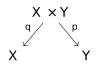
Let \(\mathcal{P}\) be a complex of sheaves in \(D^b(X\times Y)\), called a Fourier-Mukai kernel, and define the corresponding Fourier-Mukai transform \[\begin{aligned} \Phi_{\mathcal{P}}: D^b(X) &\longrightarrow D^b(Y)\\ \mathcal{E}&\longmapsto Rp_*(Lq^*\mathcal{E}\otimes^L \mathcal{P}). \end{aligned}\] We can also use the same kernel to go in the reverse direction, which we denote by \[\begin{aligned} \Phi_{\mathcal{P}}': D^b(Y) &\longrightarrow D^b(X)\\ \mathcal{E}&\longmapsto Rq_*(Lp^*\mathcal{E}\otimes^L \mathcal{P}). \end{aligned}\]
Proposition. Let \(\mathcal{O}_{\Delta}\) be the structure sheaf of the diagonal on \(X\times X\), i.e., if \(\Delta: X\to X\times_k X\) is the diagonal, \(\mathcal{O}_{\Delta} = \Delta_* \mathcal{O}_X\). Then, \[\Phi_{\mathcal{O}_\Delta} \cong 1_{D^b(X)}.\]
Proof. First, we note that \(\Delta_*\mathcal{O}_X\), considered as a degree 0 complex, coincides with \(R\Delta_* \mathcal{O}_X\) where \(\mathcal{O}_X\) is considered as a degree 0 complex, since \(\Delta\) is a closed immersion (so an affine map).
We then compute, by the derived projection formula (which is true even for non-locally free sheaves, since every complex of coherent sheaves has a locally free replacement) the following: \[\begin{aligned} \Phi_{\mathcal{O}_\Delta}(\mathcal{E}) &= Rp_*(Lq^*\mathcal{E}\otimes^L \Delta_* \mathcal{O}_X)\\ &= Rp_*(R\Delta_*(\mathcal{O}_X \otimes^L L\Delta^*Lq^* \mathcal{E}))\\ &= R(p \circ \Delta)_*(\mathcal{O}_X \otimes^L L(q\circ \Delta)^* \mathcal{E})\\ &= R(1_X)_*(\mathcal{O}_X \otimes^L L(1_X)^* \mathcal{E})\\ &= \mathcal{E} \end{aligned}\] (where all the equalities are really only natural isomorphisms). So, indeed \(\Phi_{\mathcal{O}_\Delta} \cong 1_{D^b(X)}\). ◻
Our quasi-isomorphism \(\mathcal{E}^\bullet \cong \mathcal{O}_\Delta\) then tells us, in particular, that \[\Phi_{\mathcal{E}^\bullet} \cong \Phi_{\mathcal{O}_\Delta} \cong 1_{D^b(\mathbb{P})}\] (and the same is true for the Fourier Mukai transforms in the reverse direction). In some sense, \(\mathcal{E}^\bullet\) gives us a decomposition of the identity, by replacing the single sheaf \(\mathcal{O}_\Delta\) with a complex. This will be key to proving the main theorem, which first relies on a lemma.
Lemma 2.5.
The Fourier-Mukai transforms \(\Phi_{\mathcal{E}^{-i}}'\) and \(\Phi_{\mathcal{E}^{-i}}'\) send a complex \(\mathcal{F}^\bullet\) to a direct sum of shifts of \(\mathcal{O}(-i)\) and \(\Omega^i(i)\) respectively. More specifically, \[\begin{aligned} \Phi_{\mathcal{E}^{-i}}'(\mathcal{F}^\bullet) &= \bigoplus H^j(\mathbb{P},\mathcal{F}^\bullet\otimes \Omega^i(i))[-j] \otimes_k \mathcal{O}(-i)\\ \Phi_{\mathcal{E}^{-i}}(\mathcal{F}^\bullet) &= \bigoplus H^j(\mathbb{P},\mathcal{F}^\bullet(-i))[-j] \otimes_k \Omega^i(i). \end{aligned}\]
Proof. We prove the first statement. We compute, using (1) the acyclicity of locally free sheaves for tensor and (2) the derived projection formula, that \[\begin{aligned} \Phi_{\mathcal{E}^{-i}}'(\mathcal{F}^\bullet) &= Rq_*(p^* \mathcal{F}^\bullet \otimes^L \mathcal{E}^{-i})\\ &= Rq_*(p^*\mathcal{F}^\bullet \otimes (q^* \mathcal{O}(-i) \otimes p^*\Omega^i(i)))\\ &= Rq_*(p^*(\mathcal{F}^\bullet \otimes \Omega^i(i)) \otimes q^* \mathcal{O}(-i))\\ &= Rq_*(p^*(\mathcal{F}^\bullet \otimes \Omega^i(i))) \otimes \mathcal{O}(-i). \end{aligned}\] Now, we have a fiber product square
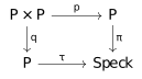
so derived flat base change tells us \[Rq_*(p^*(\mathcal{F}^\bullet \otimes \Omega^i(i))) = \tau^*(R\pi_*(\mathcal{F}^\bullet \otimes \Omega^i(i))),\] but we can identify \(R\pi_*\) with sheaf cohomology \(R\Gamma\), and \(\tau^*\) as tensoring this complex of \(k\)-vector spaces with \(\mathcal{O}_\mathbb{P}\), so we in fact get \[Rq_*(p^*(\mathcal{F}^\bullet \otimes \Omega^i(i))) = R\Gamma(\mathcal{F}^\bullet \otimes \Omega^i(i)) \otimes_k \mathcal{O}_\mathbb{P},\] and even better, \(D^b(\mathrm{Spec}k)\) has homological dimension \(\leq 1\) (\(\mathrm{Ext}^2\) and higher vanish), so a complex actually splits as a direct sum, so we can replace our \(R\Gamma\) complex with a direct sum of its cohomologies, so \[Rq_*(p^*(\mathcal{F}^\bullet \otimes \Omega^i(i))) = \bigoplus H^j(\mathcal{F}^\bullet \otimes \Omega^i(i))[-j] \otimes_k \mathcal{O}_\mathbb{P}.\] Now, plugging this into our earlier computation, we get \[\Phi_{\mathcal{E}^{-i}}'(\mathcal{F}^\bullet) = \bigoplus H^j(\mathcal{F}^\bullet \otimes \Omega^i(i))[-j] \otimes_k \mathcal{O}(-i)\] as desired. ◻
Proof of Main Theorem
Proof of Theorem 2.2. We just prove the first collection is a full strong exceptional collection—the other argument is similar.
It is not difficult to show that the first collection is strong exceptional, just standard cohomology calculations, along the lines of \[\mathrm{Hom}(\mathcal{O}(-i),\mathcal{O}(-j)) \cong \mathrm{Ext}^\ell(\mathcal{O}(-i),\mathcal{O}(-j)) \cong \mathrm{Ext}^\ell(\mathcal{O},\mathcal{O}(i-j)) \cong H^\ell(\mathcal{O}(i-j)),\] and then do case work for whether \(i<j\) or \(\ell=0,n\).
The much harder result is that this collection is full—that it generates \(D^b(\mathbb{P})\). Pick an object \(\mathcal{F}^\bullet \in D^b(\mathbb{P})\), which we will try to generate. To see this, split the exact sequence \(0\to \mathcal{E}^\bullet \to \mathcal{O}_\Delta \to 0\) into short exact sequences
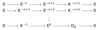
where \(\mathcal{K}^{-i} = \ker(\mathcal{E}^{-i} \to \mathcal{E}^{-i+1})\). These give distinguished triangles in \(D^b(\mathbb{P}\times \mathbb{P})\), which we can then hit with exact functors \[p^*\mathcal{F}^\bullet \otimes^L -, \qquad Rq_*\] to get the follwing distignuished triangles.
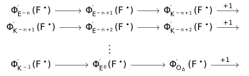
Starting from the top, we get \[\Phi_{\mathcal{K}^{-n+1}}'(\mathcal{F}^\bullet) \in \left\langle\mathcal{O}(-n),\mathcal{O}(-n+1)\right\rangle\] because it fits into a distinguished triangle where the other two terms are direct sums of shifts of \(\mathcal{O}(-n),\mathcal{O}(-n+1)\) by the lemma. The next distinguished triangle tells us \[\Phi'_{\mathcal{K}^{-n+2}}(\mathcal{F}^\bullet) \in \left\langle\mathcal{O}(-n),\mathcal{O}(-n+1),\mathcal{O}(-n+2)\right\rangle,\] and induction will get us \[\mathcal{F}^\bullet = \Phi_{\mathcal{O}_\Delta}'(\mathcal{F}^\bullet) \in \left\langle\mathcal{O}(-n),\dots,\mathcal{O}\right\rangle,\] so indeed our strong exceptional collection is actually full. ◻
Applications
Beilinson Spectral Sequence
Theorem. Given \(\mathcal{F}\in \mathrm{Coh}(\mathbb{P})\), there exist spectral sequences \[\begin{aligned} E_1^{p,q} = H^q(\mathbb{P},\mathcal{F}(p)) \otimes \Omega^{-q}(-q) & \Longrightarrow \begin{cases} \mathcal{F}& \text{if $p+q=0$}\\ 0 & \text{else} \end{cases}\\ E_1^{p,q} = H^q(\mathbb{P},\mathcal{F}\otimes \Omega^{-p}(-p)) \otimes \mathcal{O}(q) & \Longrightarrow \begin{cases} \mathcal{F}& \text{if $p+q=0$}\\ 0 & \text{else.} \end{cases} \end{aligned}\]
We first prove a lemma.
Lemma. Let \(F: \mathcal{A}\to \mathcal{B}\) be a left exact additive functor between abelian categories with enough injectives. Let \(A^\bullet \in D^+(\mathcal{A})\). Then, we have a spectral sequence \[R^qF(A^p) \Longrightarrow R^{p+q}F(A^\bullet).\]
Proof. Resolve \(A^\bullet\) with an injective double complex \(0\to A^\bullet \to I^{\bullet,\bullet}\).
Now to compute \(R^q F(A^p)\), we see that \(I^{p,\bullet}\) is an injective resolution, so this is \(H^q F(I^{p,\bullet})\), which is the vertical cohomology of the double complex \(F(I^{\bullet,\bullet})\), which forms the 1st page on the vertical spectral sequence of the double complex converging to the cohomology of the total complex \(F(I^{\bullet,\bullet})\).
On the other hand, the total complex of \(I^{\bullet,\bullet}\) is an injective complex quasi-isomorphic to \(A^\bullet\), so the \((p+q)\)th cohomology of the total complex of \(F(I^{\bullet,\bullet})\) is \(R^{p+q}F(A^\bullet)\).
Thus, we get the desired result. ◻
Proof of Theorem.. Apply the lemma for \(F=p_*\) and \(A^\bullet = q^*\mathcal{F}\otimes \mathcal{E}^\bullet\), to get spectral sequence \[\begin{aligned} R^q p_*(q^*\mathcal{F}\otimes \mathcal{E}^p) &\Longrightarrow R^{p+q} p_*(q^*\mathcal{F}\otimes \mathcal{E}^\bullet)\\ H^q \Phi_{\mathcal{E}^p}(\mathcal{F}) &\Longrightarrow H^{p+q} \Phi_{\mathcal{E}^\bullet}(\mathcal{F}), \end{aligned}\] and we apply lemma 2.5 to get the first result (and switch the roles of \(p,q\) to get the other result). ◻
Some Equivalences
Tool
To write down equivalences between triangulated categories, we’ll need the following lemma.
Definition. Let \(\mathcal{C}\) be a triangulated category. A classical generator of \(\mathcal{C}\) is an object \(C\) such that the smallest saturated (closed under direct summands) strictly full (closed under isomorphisms and contains all morphisms between given objects) triangulated subcategory of \(\mathcal{C}\) containing \(C\) is \(\mathcal{C}\) itself.
Lemma. Let \(F:\mathcal{C}\to \mathcal{D}\) be an exact functor, which sends a classical generator \(C\in \mathcal{C}\) to a classical generator \(F(C)=D\) of \(\mathcal{D}\), such that the induced map \[\mathrm{End}_{\mathcal{C}}^\bullet(C) \to \mathrm{End}_{\mathcal{D}}^\bullet(D)\] is an isomorphism. Then, \(F\) is an equivalence.
Proof. To show at least \(F\) is an equivalence, we show it is fully faithful and essentially surjective.
To see fully-faithful, first show that the full subcategory \[T_C = \{X\in \mathcal{C}\mid \text{$\mathrm{Hom}(C,X) \to \mathrm{Hom}(FC,FX)$ is a bijection}\}\] is a strictly full saturated triangulated subcategory containing \(C[i]\) for all \(i\in \mathbb{Z}\). This is true—it is clearly closed under direct sums, direct summands, and shifts. To see it is closed under cones, notice that for a distinguished triangle \(X\to Y\to Z \to X[1]\) we get a commutative diagram of (long) exact sequence

all vertical morphisms are isomorphisms except for potentially every 3rd morphism, but then we apply the 5 lemma to get \(F_{C,Z}\) is also an isomorphism. So, \(T_C\) has to be all of \(\mathcal{C}\).
The same argument shows that \[T_X' = \{Y\in \mathcal{C}\mid F_{X,Y} \text{ is bijective}\}\] is thick (since the previous step told us \(C[i]\in T_X'\)), so it is also all of \(\mathcal{C}\). This establishes that \(F\) is fully faithful.
Next, \(F\) is essentially surjective, because it is exact and has a generator in its image. Thus, \(F\) is an equivalence. ◻
Homotopy Category
The main obstacle to understanding a derived category is just how complicated morphisms are—in general I have no idea how many roofs there are. When we have enough injective/projectives, there are spectral sequences that converge to the \(\mathrm{Hom}\) groups in the derived category, but its not like spectral sequences are particularly easy either.
For \(\mathbb{P}^n\) in particular, we can take Beilinson’s argument a little further and actually get an equivalence between \(D^b(\mathbb{P}^n)\) and a homotopy category, where the morphisms are way more tractible.
First, we define some notation.
Let \(V\) be a vector space (whose elements we consider as geometric vectors), and \(V^\vee\) its dual, and set \(S= \mathrm{Sym}^\bullet V^\vee\) as usual.
Let \(\mathrm{Gr}\,S\text{-}\mathrm{Mod}\) the category of graded (left) modules over \(S_\bullet\)
Let \(M_{[0,n]}(S)\) be the full subcategory of \(\mathrm{Gr}\,S\text{-}\mathrm{Mod}\) consisting of objects which are finite direct sums of \(S(-r)\) for \(r\in \{0,\dots,n\}\).
Let \(K^b_{[0,n]}(S)\) the homotopy category of bounded complexes in \(M_{[0,n]}(S)\).
We can then define an additive functor \[\begin{aligned} M_{[0,n]}(S) &\longrightarrow \mathrm{Coh}(\mathbb{P})\\ S(-r) &\longmapsto \widetilde{S(-r)}=\mathcal{O}(-r), \end{aligned}\] which then passes to chain complex categories and then to homotopy categories (which are triangulated, by source-cylinder-cone-suspension exact triangles) \[K^b_{[0,n]}(S) \longrightarrow K^b(\mathrm{Coh}(\mathbb{P})),\] which we can post-compose with the localization functor to get \[F: K^b_{[0,n]}(S) \longrightarrow D^b(\mathbb{P}).\] In total, this functor just hits a chain complex with usual projective space sheafification/tilde, and likewise for morphisms. The left is relatively easy to understand—morphisms are homotopy classes of honest chain maps—whereas the right is a-priori difficult. The surprising thing is the following.
Theorem. The functor \(F\) is an equivalence.
Proof. The source category of \(F\) is classically generated by the object \(\bigoplus_{i=0}^n S(-i)\), the right is classically generated by \(\bigoplus_{i=0}^n \mathcal{O}(-i)\) by Beilinson. By our triangulated category lemma, and by splitting the morphism of direct sums into components, we just need to show \[\mathrm{Hom}_{K^b_{[0,n]}(S)}^\bullet(S(-i),S(-j)) \cong \mathrm{Hom}_{D^b(\mathbb{P})}^\bullet(\mathcal{O}(-i),\mathcal{O}(-j)).\] On either side, the \(\mathrm{Hom}\) groups are concentrated in degree 0—on the left because in the homotopy category we’d have no hope of writing an honest chain map, and on the right by an \(\mathrm{Ext}\) computation. So, we only have to worry about degree 0 homomorphisms, but this is straightforward—we will get \[\mathrm{Hom}(S(-i),S(-j)) = \mathrm{Hom}(S,S(i-j) = \mathrm{Sym}^{i-j} V^\vee = \Gamma(\mathcal{O}(i-j)) = \mathrm{Hom}(\mathcal{O}(-i),\mathcal{O}(-j)).\] ◻
Remark. We will get an analogous equivalence corresponding to the \(\mathcal{O},\Omega^1(1),\dots,\Omega^n(n)\) full strong exceptional collection.
Define \(K_{[0,n]}^b(E)\) to be the homotopy category of bounded complexes valued in finite direct sums of \(E(-r)\) (with \(r=0,\dots,n\)) where \(E=\bigwedge^\bullet V\).
Then, we get a functor \[F': K_{[0,n]}^b(E) \longrightarrow D^b(\mathbb{P}^n)\] which interprets \(E(-r)\) as \(\Omega^r(r)\).
Quiver Representations
Unlike the previous equivalence, the following goes through whenever we have an exceptional collection. We’ll see specifically how this works for \(\mathbb{P}^n\).
Definition. Let \(X\) be a smooth projective variety over \(k\). A sheaf \(T\in \mathrm{Coh}(X)\) is called a tilting sheaf if
the algebra \(A:=\mathrm{End}(T)\) has finite global dimension (i.e., there exists \(d\in \mathbb{Z}_{\geq 0}\) such that any module admits a projective resolution of length less than \(d\)).
The modules \(\mathrm{Ext}^\ell(T,T)=0\) for all \(\ell>0\).
The object classically generates \(D^b(X)\), i.e., the smallest strictly full saturated (closed under direct summands) triangulated subcategory containing \(T\) is \(D^b(X)\).
Proposition. Let \(E_1,\dots,E_r \in \mathcal{A}\) be a full strong exceptional collection for \(D^b(\mathcal{A})\). Then, \[T = \bigoplus_{i=1}^r E_i\] is a tilting object.
We’re approaching a result which tells us how nice a tilting sheaf is—in the same way the triangulated category generated by a single exceptional object is just \(D^b(k)\), we’ll see that the triangulated category generated by a tilting sheaf is \(D^b(\mathrm{mod}\text{-}A)\).
Theorem 3.9.
Let \(T\) be a tilting sheaf on a projective smooth \(X\) over \(k\), with \(A=\mathrm{End}(T)\). Then, the following functors form an equivalence. \[\begin{aligned} RG= \mathrm{RHom}(T,-): D^b(X) &\longrightarrow D^b(\mathrm{mod}\text{-}A)\\ LF= - \otimes_A^L T: D^b(\mathrm{mod}\text{-}A) &\longrightarrow D^b(X) \end{aligned}\]
Proof. First, we more carefully define the functors.
We have the left exact functor \(G=\mathrm{Hom}(T,-): \mathrm{QCoh}(X) \to k\text{-}\mathrm{Vec}\), which actually factors through \(\mathrm{Mod}\text{-}A\) because we have an action by precomposition.
The category \(\mathrm{QCoh}(X)\) has enough injectives, so we can right derive the functor to get \[\mathrm{RHom}(T,-): D^+(\mathrm{QCoh}(X)) \to D^+(\mathrm{Mod}\text{-}A),\] and usual arguments tell us that this descends to \[RG = \mathrm{RHom}(T,-): D^b(X) \to D^b(\mathrm{mod}\text{-}A),\] (we have an Ext spectral sequence to ensure that we get bounded complexes because \(\mathrm{Coh}(X)\) has finite global dimension, and morphisms between coherent sheaves are finite dimensional to ensure that precomposed with \(D^b(X) \cong D^b_{\mathrm{Coh}(X)}(\mathrm{QCoh}(X)) \hookrightarrow D^b(\mathrm{QCoh}(X))\) will with us finitely generated \(A\) modules).
In the other direction, we have the functor \[F = - \otimes_A T: \mathrm{mod}\text{-}A \to \mathrm{QCoh}(X),\] in the following sense.
that given \(M \in \mathrm{mod}\text{-}A\), we get then \(\underline{M}\) is in \(\mathrm{Mod}\text{-}\underline{A}\) and \(T\) is in \(\underline{A} \text{-}\mathrm{Mod}\), so we can form the \(\underline{A}\)-balanced tensor product, which is then inherits an \(\mathcal{O}_X\)-module structure from \(T\) (via left multiplication).
This functor is right exact, and \(\mathrm{mod}\text{-}A\) has enough projectives, so we can left derive it to get \[- \otimes_A^L T: D^-(\mathrm{mod}\text{-}A) \to D^-(\mathrm{QCoh}(X)),\] and Serre theorems/finite global dimension of \(A\) will give sheaf Tor finite dimensions/vanishing to imply that this functor descends to \[LF = - \otimes_A^L T: D^b(\mathrm{mod}\text{-}A) \to D^b(X).\]
Now, we need to show these functors form an equivalence. The assumption T2 for \(T\) exactly tells us that \(RG(T)=A\), and so we also get a (ring) morphism \[\mathrm{End}^\bullet(T) \xrightarrow{RF} \mathrm{End}^\bullet(A),\] which is an isomorphism because in nonzero degrees both sides are 0 (by Ext vanishing or because \(A\) is projective), and then in degree 0, it sends an endomorphism \(f:T\to T\) to left multiplication by \(f\in A\), which are exactly the endomorphisms of \(A\) as a right \(A\)-module.
So, our lemma tells us that \(RG\) is an equivalence, but a-priori we do not know that \(LF\) is a quasi-inverse. To see this, we first notice that \(F\dashv G\) form an adjunction before we derived anything. To see this (it seems slightly subtle because it varies slightly from usual tensor-hom in the sheafiness of it), we will spell out the unit and counit, and check the triangle identities. We have \(\eta: 1_{\mathrm{Mod}\text{-}A} \Rightarrow GF\) by \[\eta_M: M \to \mathrm{Hom}(T,M\otimes_A T)\] where we send \(m\) to the morphism \(t\mapsto m\otimes t\) (which first is a map to the tensor presheaf, but then we postcompose to get a map to the sheafification). Then, we have \(\varepsilon: FG \Rightarrow 1_{\mathrm{QCoh}(X)}\) by \[\varepsilon_\mathcal{E}: \mathrm{Hom}(T,\mathcal{E}) \otimes_A T \to \mathcal{E}\] where we send \(\phi \otimes t\) to \(\phi(t)\) (which is a map from the presheaf factoring through the sheafification). Then, one checks that the triangle identities hold by computing the compositions on stalks—where sheafification is not a concern. ◻
We gave an equivalence \(D^b(X) \cong D^b(\mathrm{mod}\text{-}A)\), but \(\mathrm{mod}\text{-}A\) turns out to be a very concrete category—we will recognize \(A\) to be a quiver algebra \(kQ/I\), so that \[\mathrm{mod}\text{-}A \cong A^\mathrm{op}\text{-}\mathrm{mod}\cong \mathrm{rep}(Q^\mathrm{op},I^\mathrm{op}).\]
To see the quiver, we write more suggestively \(A\) as the algebra of matrices \[\begin{bmatrix} \mathrm{Hom}(E_1,E_1)=k & \mathrm{Hom}(E_1,E_2) & \cdots & \mathrm{Hom}(E_1,E_n)\\ 0 & \mathrm{Hom}(E_2,E_2)=k & \cdots & \mathrm{Hom}(E_2,E_n)\\ \vdots & \vdots & \ddots & \vdots\\ 0 & 0 & \cdots & \mathrm{Hom}(E_n,E_n)=k \end{bmatrix}\] with multiplication given by matrix multiplication/composition of Homs.
The Jacobson radical \(J\) of \(A\) will be the strictly upper triangular matrices in our suggestive matrix. To see this, set \(J\) the direct sum of all Homs which are not \(\mathrm{Hom}(E_i,E_i)\) (the strictly upper triangular matrices), and check (via (Assem, Simson, and Skowroński 2006, I.1.4)) that \(J\) is nilpotent and \(A/J\) is a product of copies of \(\mathbb{C}\).
First, \(J\) is nilpotent because \(J^\ell\) only consists of formal sums of morphisms \(E_i\to E_{i+\ell}\), so when \(\ell\geq r\), there are no more morphisms to sum over.
Next, \(A/J\) is isomorphic to \[\prod_{i=1}^r \mathrm{Hom}(E_i,E_i) = \prod_{i=-n}^0 \mathbb{C},\] so indeed a product of fields.
The Jacobson radical is really the tool to find the quiver \(Q\). We set the vertices of \(Q\) to be a chosen basis for \(A/J\), so conveniently we’ll choose the basis to be \(\mathrm{id}_{E_1},\dots,\mathrm{id}_{E_r}\). Next, we set the arrows from \(E_i\) to \(E_j\) to be a chosen basis for \(\mathrm{id}_{E_j} (J/J^2) \mathrm{id}_{E_i}\).
Example. Let’s understand for \[A = \mathrm{End}(\bigoplus_{i=-n}^{0} \mathcal{O}(i))\] how to see \(A\) as a bound quiver algebra. Our suggestive matrix is the following. \[\begin{bmatrix} k\cdot \mathrm{id}_{\mathcal{O}(\text{-}n)} & \mathrm{Hom}(\mathcal{O}(\text{-}n),\mathcal{O}(\text{-}n+1)) & \cdots & \mathrm{Hom}(\mathcal{O}(\text{-}n),\mathcal{O})\\ 0 & k \cdot \mathrm{id}_{\mathcal{O}(\text{-}n+1)} & \cdots & \mathrm{Hom}(\mathcal{O}(\text{-}n+1),\mathcal{O})\\ \vdots & \vdots & \ddots & \vdots\\ 0 & 0 & \cdots & k\cdot \mathrm{id}_{\mathcal{O}} \end{bmatrix}= \begin{bmatrix} k & k^{\binom{n+1}{1}} & \cdots & k^{\binom{n+n}{n}}\\ 0 & k & \cdots & k^{\binom{n+n-1}{n-1}}\\ \vdots & \vdots & \ddots & \vdots\\ 0 & 0 & \cdots & k \end{bmatrix}\] As explained earlier, \(J\) is the upper triangular matrices. To compute the arrows from \(\mathcal{O}(i)\) to \(\mathcal{O}(j)\), we compute \[\mathrm{id}_{\mathcal{O}(j)} (J/J^2) \mathrm{id}_{\mathcal{O}(i)} = \mathrm{id}_{\mathcal{O}(j)}J \mathrm{id}_{\mathcal{O}(i)}/ \mathrm{id}_{\mathcal{O}(j)} J^2 \mathrm{id}_{\mathcal{O}(i)}.\] As a first step, we compute \(\mathrm{id}_{\mathcal{O}(j)} J \mathrm{id}_{\mathcal{O}(i)}\), which is exactly \(\mathrm{Hom}(\mathcal{O}(i),\mathcal{O}(j))\). Next, we compute \[\mathrm{id}_{\mathcal{O}(j)} J^2 \mathrm{id}_{\mathcal{O}(i)},\] which will be the subset of \(\mathrm{Hom}(\mathcal{O}(i),\mathcal{O}(j))\) that factor as a sum of maps which go through some strictly intermediate \(\mathcal{O}(\ell)\). If \(j=i+1\), then no strict factorization is possible. If \(j>i+1\), then we always have a strict factorization, since a map \(\mathcal{O}(i)\to \mathcal{O}(j)\) will be given by a degree \(j-i\) homogeneous polynomial, which we can write as a sum of monomials, and then peeling one monomial away we get the factorization.
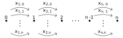
So, \[\mathrm{id}_{\mathcal{O}(j)} (J/J^2) \mathrm{id}_{\mathcal{O}(i)} \cong \begin{cases} \mathrm{Hom}(\mathcal{O}(i), \mathcal{O}(i+1)) & j=i+1\\ 0 & \text{otherwise.} \end{cases}\] Therefore, we should place \(n+1\) arrows between \(\mathcal{O}(i)\) and \(\mathcal{O}(i+1)\) for a chosen basis \[\mathrm{Hom}(\mathcal{O}(i),\mathcal{O}(i+1)) = \left\langle x_{i,0},\dots,x_{i,n}\right\rangle.\]
So far, we have the quiver \(Q\), now we want to compute the relations, so we study the natural map \[kQ \to A\] given by the universal property of quiver algebras (Assem, Simson, and Skowroński 2006, II.1.8), and we find a generating set of the kernel. We claim that the kernel is generated by terms \[R=\{x_{i+1,p}x_{i,q} - x_{i+1,q}x_{i,p} \mid 0\leq p,q \leq n, -n \leq i \leq 0\}.\] We can see that all of \(R\) is in the kernel, since \[x_{p}x_{q} = x_{q}x_{p} \in \mathrm{Hom}(\mathcal{O}(i),\mathcal{O}(i+2)).\] Now, we check that \(\left\langle R\right\rangle\) is the entire kernel by seeing that \(kQ/\left\langle R\right\rangle \to A\) is injective. In fact, both \(k\)-algebras here are graded by lengths of paths, so we can show the kernel is 0 by showing each graded piece is 0.
Suppose \[\sum \alpha_{p_0,\dots,p_r} x_{i+r,p_r} \cdots x_{i,p_0} \in (kQ/\left\langle R\right\rangle)_r\] is in the kernel, i.e., \[\sum \alpha_{p_0,\dots,p_r} x_{p_r} \cdots x_{p_0} = 0 \in \mathrm{Hom}(\mathcal{O}(i),\mathcal{O}(i+r)) = k[x_0,\dots,x_n]_r,\] i.e., it is the zero polynomial. This will imply our original term in \(kQ/\left\langle R\right\rangle\) is 0, since we can use \(R\) to put all the monomials in standard order.
In conclusion, we get that \(A\) is the algebra for the (bound) Beilinson \(\mathbb{P}^n\) quiver, i.e., the quiver
with the relations \[x_{p,i+1}x_{q,i} - x_{q,i+1}x_{p,i} = 0.\]