Brauer Group
April 2026
The Brauer group of a scheme \(X\) (and its mild variations) is a gadget that has diverse applications:
algebras: it parameterizes sheaves of Azumaya algebras (generalizing the classical Brauer group),
cohomology: it is a cohomological invariant, by being a “higher” version of the Picard group, i.e., going from \(H^1_{\mathrm{\acute{e}t}}(X,\mathbb{G}_m)\) to \(H^2_\mathrm{\acute{e}t}(X,\mathbb{G}_m)\) (in fancier language, going from “torsors” to “gerbes”).
obstructions: it obstructs (étale) projective bundles from lifting to vector bundles, as well as often obstructing universal families on coarse moduli spaces.
noncommutative geometry: Brauer classes twist the category of coherent sheaves, providing some of the most concrete “noncommutative” spaces of concern in algebraic geometry.
The main focus of our series of talks will be to show how this one gadget has all of these features.
Brauer Group of a Field
Overview and Definitions
We start by defining the Brauer group.
Definition. A central simple algebra (CSA) over a field \(k\) is an algebra \(A\) over \(k\) with \(Z(A)=k\) and no nontrivial proper two-sided ideals (so a-priori only simple in the category of algebras, not modules).
Two CSAs \(A\), \(B\) are called similar if for some \(n,m\in \mathbb{N}\), \[A \otimes_k M_n(k) \cong B \otimes_k M_m(k)\] (which turns out to be identical to Morita equivalence, i.e., \(A\text{-}\mathrm{mod}\cong B\text{-}\mathrm{mod}\)).
The Brauer group of \(k\) is \[\mathrm{Br}(k) :=\{A \text{ central simple algebra}/k\} / \text{similarity},\] which turns out to be a group under \(\otimes_k\) (check that a CSA \(A\) is tensor invertible up to similarity by seeing that \(A\otimes_k A^\mathrm{op}\sim k\)).
This is already a very interesting object, ask any number theorist. Especially interesting are the following cohomological characterization, in terms of group/Galois cohomology, which we will define later. This first characterization in particular is very tractible and useful for computation.
Theorem 1.2.
\(\mathrm{Br}(k) \cong H^2(k,k^\times) :=H^2_{\text{cont}}(\mathrm{Gal}(k_{\text{sep}}/k),k_{\text{sep}}^\times)\).
How, to prove the first one, we first go through the following result.
Proposition. \(\mathrm{Br}(k) \cong H^1(k,\mathrm{PGL}_\infty) :=H^1_{\text{cont}}(\mathrm{Gal}(k_\text{sep}/k),\mathrm{PGL}_\infty(k_\text{sep}))\).
Before we sketch these proofs, we review definitions of these \(H^i_{\text{cont}}\) objects. To start, we define group cohomology, before giving even more specific definitions.
Review of Group Cohomology
For a group \(G\) and a \(\mathbb{Z}[G]\)-module \(A\), which is the data of an abelian group \(A\) together with a \(\mathbb{Z}\)-linear \(G\)-action, i.e., a morphism \[G\to \mathrm{Aut}_\mathbb{Z}(A)\] where we denote the action of \(g\in G\) on \(a\in A\) by \(g(a)\).
We will spend some time to review group cohomology, and spell out the first cohomology group. In fact, we will see that at least the first cohomology makes sense as a pointed set, even when \(A\) is not abelian (it just has a left \(G\)-action), which is a case we will need to consider.
By definition, group cohomology (with coefficients in an abelian group with linear \(G\)-action) is the derived functor of invariants \((-)^G\), and the invariants functor is naturally isomorphic to \(\mathrm{Hom}_{\mathbb{Z}[G]}(\mathbb{Z},-)\) where \(\mathbb{Z}\) has the trivial \(G\)-action, so \[H^1(G,A) = \mathrm{Ext}^1(\mathbb{Z},A),\] and we can compute by first writing down a projective resolution of \(\mathbb{Z}\). For a group \(G\), there is the bar resolution of \(\mathbb{Z}\) (with the trivial \(G\)-action) by \[\left( \cdots \to \mathbb{Z}[G^3] \to \mathbb{Z}[G^2] \to \mathbb{Z}[G] \right) \xrightarrow{\sim_{\text{qis}}} \mathbb{Z}\to 0\] sending \[[g_0|g_1|\cdots|g_n] \mapsto \left(\sum_{i=1}^n (-1)^{i+1} [g_0|g_1|\cdots|g_{i-1}g_i|\cdots|g_n]\right) + (-1)^n [g_0|g_1|\cdots|g_{n-1}]\] (coming from the monad of the extension/restriction of scalars adjunction along the ring inclusion \(\mathbb{Z}\to \mathbb{Z}[G]\), i.e., take alternating sums of whiskered counit maps \(LR\Rightarrow 1\)). Therefore, \(H^1(G,A)\) is the cohomology of the complex \[\mathrm{Hom}_{\mathbb{Z}[G]}(\mathbb{Z}[G],A) \to \mathrm{Hom}_{\mathbb{Z}[G]}(\mathbb{Z}[G^2], A) \to \mathrm{Hom}_{\mathbb{Z}[G]}(\mathbb{Z}[G^3], A).\] Noting that each of the left \(\mathbb{Z}[G]\)-modules are free, on generators \(1,G,G^2\) respectively, we use the free-forget adjunction to consider this as a sequence \[\mathrm{Hom}_\mathrm{Set}(\{*\},A) \xrightarrow{d^0} \mathrm{Hom}_\mathrm{Set}(G,A) \xrightarrow{d^1} \mathrm{Hom}_\mathrm{Set}(G^2,A),\] and we can compute the differentials as follows (where we denote a function \(G^n\to A\) as an indexed tuple \(a_{(-,\dots,-)}\)). Note that we are writing the abelian group operation for \(A\) multiplicatively. For \(d^1\), recall that the degree 2 bar resolution map (on a generator) is \[\begin{aligned} &\mapsto [\sigma|\tau] - [1|\sigma\tau] + [1|\sigma]\\ &= \sigma[1|\tau] - [1|\sigma\tau] + [1|\sigma]. \end{aligned}\] Therefore, the pullback map is given by \[\begin{aligned} d^1: \mathrm{Hom}_\mathrm{Set}(G,A) &\longrightarrow \mathrm{Hom}_\mathrm{Set}(G^2,A)\\ a_{(-)} &\longmapsto ((\sigma,\tau) \mapsto \sigma(a_{\tau})) (a_{\sigma\tau})^{-1} a_{\sigma}, \end{aligned}\] so the cocycles (the elements of the kernel) are given by the preimage of \((\sigma,\tau)\mapsto 1\) in \(\mathrm{Hom}_\mathrm{Set}(G^2,A)\), which is exactly given by \[\{a_{(-)} \mid a_{\sigma\tau} = a_\sigma \sigma(a_\tau) \text{ for all $\sigma,\tau\in G$}\}.\] Next, recall that the degree 1 bar resolution map (on a generator) is \[[1|\sigma] \mapsto [\sigma] - [1],\] so the pullback map is given by (denoting \(c\) the image of \(*\) under a set map \(\{*\}\to A\)) \[\begin{aligned} d^0: \mathrm{Hom}_\mathrm{Set}(\{*\},A) &\longrightarrow \mathrm{Hom}_\mathrm{Set}(G,A)\\ c &\longmapsto (\sigma \mapsto \sigma(c)c^{-1}), \end{aligned}\] so the coboundaries are \(A\)-orbit maps.
Therefore, two cocycles \(a_{(-)}\) and \(b_{(-)}\) are cohomologous if there exists \(c\in A\) such that \[\begin{aligned} b_{\sigma}a_{\sigma}^{-1} &= \sigma(c)c^{-1}, \end{aligned}\] which is straightforward in the abelian/commutative setting, but for some reason (which we will see when we define twisted forms) the best way to write this so that we can generalize to the nonabelian setting, is to instead write \[a_\sigma = c^{-1} b_\sigma \sigma(c)\] (which agrees with above in when everything commutes).
In this way, we can always define, even for \(A\) nonabelian, \[H^1(G,A) :=\{1-cocyles\}\big/ \text{cohomology equiv. relation},\] and this carries a natural basepoint which is the cohomology class represented by the cocycle \[\begin{aligned} G&\to A\\ g &\mapsto 1. \end{aligned}\]
More Specialized Definitions
Now that we have a handle on group cohomology, we spell out the remaining terms in Theorem 1.2.
\(k_\text{sep}\) is the separable closure of \(k\), i.e., it is the largest separable extension of \(k\) inside \(\overline{k}\) (so if \(k\) is perfect, then \(k_\text{sep}=\overline{k}\)).
\(H^2(k,k_\text{sep}^\times)\) is the Galois cohomology, which is by definition the (continuous) group cohomology written on the right.
\(H^2_{\text{cont}}(\mathrm{Gal}(k_{\text{sep}}/k),k_{\text{sep}}^\times)\) is continuous group cohomology since the (absolute) Galois group is in general/usually infinite, and we should remember its profinite topology, which comes from recognizing that \(\mathrm{Gal}(k_\text{sep}/k)\) is the inverse limit of all of the restriction maps \(\mathrm{Gal}(k''/k) \to \mathrm{Gal}(k'/k)\) for \(k\leq k' \leq k''\) a tower of finite Galois extensions.
In general...
Definition. A profinite group \(G\) is an inverse limit of finite groups \(G_\alpha\), i.e., \[G = \varinjlim G_\alpha\] and \(G\) has a natural topology by considering each \(G_\alpha\) to have the discrete topology, and identifying the inverse limit as a subspace \[G \subseteq \prod_\alpha G_\alpha,\] where the product has the product topology.
Remark. The inverse limit is a closed topological subgroup of \(\prod G_\alpha\), it is compact and totally disconnected, and the open subgroups are exactly the closed subgroups of finite index.
One advantage of remembering the profinite topology on a Galois group of an infinite extension, is we get a generalization of the usual Galois correspondence:
Theorem. There is a bijection between subextensions of \(K/k\) and closed subgroups of \(\mathrm{Gal}(K/k)\).
Definition. A continuous \(G\)-module \(A\) is one such that the \(G\)-action is continuous, or equivalently the stabilizer of each \(a\in A\) is open in \(G\).
We will eventually define continuous group cohomology as a certain direct limit of (usual) group cohomologies of \(G_\alpha\) valued in certain coefficients coming from \(A\). We will need to understand
How to restrict coefficients along a quotient map.
How to map from group cohomology of a restriction by inflation maps.
Step 1. Given a surjection \(G\to G/H\) (thinking one of the maps \(G_\beta \to G_\alpha\) in the inverse system), and a \(G\)-module \(A\), we should find natural \(G/H\)-module coming from \(A\). The fixed points \(A^H\) is a \(G\)-submodule where \(H\) acts trivially, so the \(G\)-action descends to a \(G/H\) action.
Step 2. We will construct a natural morphism \[H^i(G/H, A^H) \to H^i(G, A)\] called an inflation map. This can be written very concretely by talking about projective resolutions in \(\mathbb{Z}[G]\text{-}\mathrm{Mod}\) versus \(\mathbb{Z}[G/H]\text{-}\mathrm{Mod}\), but we instead give an abstract derived category description.
Recall that these group cohomologies are just the cohomologies of objects \[\mathrm{RHom}_{\mathbb{Z}[G/H]\text{-}\mathrm{Mod}}(\mathbb{Z}_{G/H}, A^H), \quad \mathrm{RHom}_{\mathbb{Z}[G]\text{-}\mathrm{Mod}}(\mathbb{Z}_G, A)\] which are both objects of \(D(\mathbb{Z}\text{-}\mathrm{Mod})\) (where we subscript \(\mathbb{Z}\) by \(G/H\) or \(G\) to indicate that this is the restriction of scalars of along a morphism \(\mathbb{Z}[G]\to \mathbb{Z}[G/H]\to \mathbb{Z}\)). This inflation map is really a map in this derived category. First, recognize that \[\mathbb{Z}_{G/H} \cong \mathbb{Z}_G \otimes_{\mathbb{Z}[G]} \mathbb{Z}[G/H] \cong \mathcal{H}^0(\mathbb{Z}_G \otimes^L_{\mathbb{Z}[G]} \mathbb{Z}[G/H]),\] and recall that there is a truncation map to the 0th homology \[\mathbb{Z}_G \otimes^L_{\mathbb{Z}[G]} \mathbb{Z}[G/H] \xrightarrow{\tau} \mathcal{H}^0(\mathbb{Z}_G \otimes^L_{\mathbb{Z}[G]} \mathbb{Z}[G/H])\] in the derived category, so we have a morphism \[\mathrm{RHom}_{\mathbb{Z}[G/H]\text{-}\mathrm{Mod}}(\mathbb{Z}_{G/H}, A^H) \xrightarrow{\tau^*} \mathrm{RHom}_{\mathbb{Z}[G/H]\text{-}\mathrm{Mod}}(\mathbb{Z}_{G} \otimes^L_{\mathbb{Z}[G]} \mathbb{Z}[G/H], A^H),\] after which we can apply the extension/restriction of scalars adjunction to get a morphism \[\mathrm{RHom}_{\mathbb{Z}[G/H]\text{-}\mathrm{Mod}}(\mathbb{Z}_{G} \otimes^L_{\mathbb{Z}[G]} \mathbb{Z}[G/H], A^H) \cong \mathrm{RHom}_{\mathbb{Z}[G]\text{-}\mathrm{Mod}}(\mathbb{Z}_{G}, A^H),\] (since \(A^H\) restricted to \(\mathbb{Z}[G]\) is what we had already been calling \(A^H\)), and then we can postcompose along the inclusion \(A^H\to A\) to finally get our map to \[\mathrm{RHom}_{\mathbb{Z}[G]}(\mathbb{Z}_G, A).\] Composing all of these maps and taking cohomology objects, we get our inflation map on group cohomology.
Definition. The continuous group cohomology of profinite group \(G=\varprojlim G_\alpha\) with coefficients in a continuous \(G\)-module \(A\) is the following direct limit: along surjections \(\phi_{\alpha\beta}: G_\beta \to G_\alpha\) defining the inverse system for \(G\), get inflation maps \[\mathrm{Inf}_\alpha^\beta: H^i(G_\alpha, A^{U_\alpha}) \to H^i(G_\beta, A^{U_\beta})\] which define a directed system, and then denote \[H_{\text{cont}}^i(G,A) :=\varinjlim H^i(G_\alpha,A^{U_\alpha}).\]
Finally, this is the sense in which the Brauer group is a (continuous) group cohomology.
Proof Sketch for \(H^1\) Characterization
Now, we move on towards proving our stated theorems/propositions.
The sketch is as follows (and we will fill in the details):
Work in a relative setting, only studying CSAs split by a finite field extension \(K/k\).
Classifying such CSAs of a given dimension/degree by a nonabelian cohomology set \(H^1(\mathrm{Gal}(K/k), \mathrm{PGL}_n(K))\).
Realizing that all Morita equivalence classes of \(K\)-split CSAs are given by taking a direct limit over \(n\), denoted \(H^1(\mathrm{Gal}(K/k), \mathrm{PGL}_\infty(K))\).
Taking a direct limit over \(K/k\) separable to get \(\mathrm{Br}(k)\) as \(H^1_{\text{cont}}(\mathrm{Gal}(k_\text{sep}/k), \mathrm{PGL}_\infty(k_\text{sep}))\).
Splitting CSAs
Proposition. Let \(A\) be a finite dimensional \(k\)-algebra, and \(K/k\) a finite extension. Then, \(A\) is central simple over \(k\) iff \(A\otimes_k K\) is central simple over \(K\).
In fact, we can choose \(K\) “large” enough such that the following holds.
Proposition. There exists a finite extension \(K/k\) such that \(A\otimes_k K \cong M_n(K)\).
In particular, \(\dim_k A\) is square, since for such a field extension \(K/k\), taking \(k\)-dimensions we get \[\dim_k A \cdot [K: k] = [K: k]\cdot n^2,\] and we call this \(n\) the degree of the CSA over \(k\).
We call such a field extension a splitting field for \(A\). Note if \(F/K/k\) is a tower of field extensions, and \(K\) is a splitting field for \(A\), then so is \(F\) because \[A\otimes_k F \cong (A\otimes_k K) \otimes_K F \cong M_n(K)\otimes_K F \cong M_n(F),\] and in fact a separable splitting field always exists.
Proposition 1.11 (Noether, Köthe).
Every central simple algebra \(A\) over \(k\) has a splitting field for \(A\) which is separable over \(k\).
So, every CSA is split over \(k_\text{sep}\).
Classifying split CSAs of a fixed degree
For the sake of finiteness, fix a finite Galois extension \(K/k\) (and we will take direct limits/unions later). We will instead first try to characterize \[\mathrm{Br}(K/k) = \{\text{CSAs$/k$ split over $K$}\}/\text{Morita equivalence},\] where we work one degree at a time. Denote \[\mathrm{CSA}_k(n) :=\{\text{CSAs over $k$ split over $K$ of degree $n$}\}/\text{isomorphism}.\] Note that Morita equivalent CSAs of the same \(k\)-dimension are actually isomorphic (by the alternate characterization of Morita equivalence for CSAs).
We want to characterize this cohomologically, but unfortunately we will need to step outside of the abelian category world and use nonabelian cohomology sets, as defined in the first section.
We will then show that there is a base-point preserving bijection \[\mathrm{CSA}_{K|k}(n) \leftrightarrow H^1(\mathrm{Gal}(K/k),\mathrm{PGL}_n(K)).\]
This is the hardest and probably most important step. We abstract to a more general setup.
Definition. Let \(V\) be a \(k\)-vector space, a \(\Phi\) a tensor of type \((p,q)\) where \(p,q\in \mathbb{N}\), i.e., \[\Phi \in V^{\otimes p} \otimes_k (V^*)^{\otimes q}.\]
An isomorphism of pairs \((V,\Phi)\to (W,\Psi)\) is a \(k\)-isomorphism \(f:V\to W\) with \[f^{\otimes q} \otimes (f^{*-1})^{\otimes q}\] maps \(\Phi\) to \(\Psi\).
Remark. If we regard the space of \((p,q)\)-tensors as \[\mathrm{Hom}(V^{\otimes q}, V^{\otimes p}),\] then the condition for being an isomorphism of pairs can also be expressed as a commutative diagram
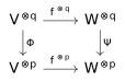
which makes sense even when \(f\) is not an isomorphism. This also makes it clear, that in the special case that \(q=2,p=1\), such an \(f\) is a \(k\)-algebra isomorphism.
We can then base change a pair \((V,\Phi)\) along a field extension \(K/k\), which we denote \((V_K, \Phi_K)\), we say that pairs \((V,\Phi),(W,\Psi)\) become isomorphic over \(K\) if their base changes become isomorphic.
Definition. Fixing a pair \((V,\Phi)\), if \((W,\Psi)\) becomes isomorphic to it over \(K\), we call then say \((W,\Psi)\) is a \((K/k)\)-twisted form of \((V,\Phi)\), or a twisted form for short. Denote the set of twisted forms by \[\mathrm{TF}_K(V,\Phi).\]
In this way, to calculate \(\mathrm{CSA}_{K|k}(n)\), we want to parameterize all \(k\)-isomorphism classes of \(K/k\)-twisted forms of \[(M_n(k),\text{matrix mult.}),\]
where one should check that such a twisted form is automatically a CSA (i.e., multiplication is still associative with unit, the center is still \(k\), and the algebra is still simple).
Going back to the general theory, we parameterize each \(k\)-isomorphism class of \((K/k)\)-twisted forms by Galois theory. The strategy is to prove the following proposition.
Proposition. \(\mathrm{TF}_K(V,\Phi) \leftrightarrow H^1(\mathrm{Gal}(K/k),\mathrm{Aut}_K(\Phi))\).
Proof Sketch. First, given a twisted \(K\)-form, encoded by a \(K\)-isomorphism \(f\) from our fixed \((V_K,\Phi_K)\) to another \((W_K,\Psi_K)\), we will produce a 1-cocycle, which is a certain type of set function \[a_{(-)}: \mathrm{Gal}(K/k) \to \mathrm{Aut}_K(\Phi)\] by \[a_\sigma :=f^{-1} \circ \sigma(f),\] where \(\sigma(f)\) means conjugating \(f\) by \(\sigma\), which we are identifying with \(1\otimes \sigma \in \mathrm{Aut}(V\otimes_k K)\), to get in total \[f^{-1} \circ \sigma \circ f \circ \sigma^{-1},\] ( this looks like a commutator?), and one checks that this is a 1-cocycle (and this only depends on \((W,\Psi)\), not the choice of isomorphism \(f\)). One then passes to the cohomology class of the cocycle.
The converse direction works more generally. Given a group \(G\) acting on a group \(A\) acting on a set \(X\) (so in our example, \(G=\mathrm{Gal}(K/k)\), \(A=\mathrm{Aut}_K(\Phi)\), and \(X=V_K\)), we take as input a \(1\)-cocycle \(a_{(-)}\) of \(G\) with coefficients in \(X\), and we produce a twisted \(G\)-action on \(X\). Even better, if \(X\) has extra structure and \(A\) acts by automorphisms, then the twisted \(G\)-action will as well—so in our setup, we will go from a 1-cocycle \[a_{(-)} \in H^1(\mathrm{Gal}(K/k),\mathrm{Aut}_K(\Phi))\] to a twisted \(G\)-action \[G\to \mathrm{Aut}_K(\Phi)\] which we denote \({}_a V_K\). Then, we will see that the invariant space \[({}_a V_K)^G\] yields a twisted form of \((V,\Phi)\), and you get isomorphic twisted forms cohomologous cocycles.
Finally, one should show that these processes are inverse to each other. ◻
So far, the proposition gives us \[\mathrm{CSA}_{K|k}(n) \leftrightarrow \mathrm{TF}_K(M_n(k),\text{matrix mult.}) \leftrightarrow H^1(\mathrm{Gal}(K/k), \mathrm{Aut}_K(M_n(K))),\] (where we mean automorphisms of the \(K\)-algebra, not \(K\)-vector space), so the remaining step is to show \(\mathrm{Aut}_K(M_n(K)) \cong \mathrm{PGL}_n(K)\).
Proposition (Skolem-Noether). Every \(K\)-algebra automorphism of \(M_n(K)\) are inner, i.e., given by conjugation with some invertible matrix \(C\).
Corollary. The automorphism group of \(M_n(K)\) is the projective general linear group \(\mathrm{PGL}_n(K)\).
Proof. By the Skolem-Noether theorem, the map \[\begin{aligned} \mathrm{GL}_n(K) &\to \mathrm{Aut}(M_n(K))\\ C &\longmapsto (M\mapsto CMC^{-1}) \end{aligned}\] is surjective, and as usual for conjugation, the kernel is exactly the center of \(\mathrm{GL}_n(K)\), which is \(K^* \hookrightarrow \mathrm{GL}_n(K)\) as diagonal matrices. ◻
Thus, we indeed get \[\mathrm{CSA}_{K|k}(n) \leftrightarrow H^1(\mathrm{Gal}(K/k), \mathrm{PGL}_n(K)).\]
Take the limit \(n\to \infty\)
There is a natural map \[\mathrm{CSA}_k(n) \to \mathrm{CSA}_k(nm)\] which is sending \(A\mapsto A\otimes_k M_m(k)\), and you can prove that this is injective.
So, the moral is that by Proposition 1.11, every CSA appears for a sufficiently large \(n\), and given any finite set of CSAs of degrees \(n_1,n_2\dots,n_r\), each of their Morita equivalences classes will have unique representatives in \(\mathrm{CSA}_k(n_1 n_2\cdots n_r)\). So, we get the entire Brauer group (split by \(K/k\)) by taking the direct limit of all of these inclusions.
On the other side, from the inclusion of \(\mathrm{GL}_n \hookrightarrow \mathrm{GL}_{mn}\) as \(m\) copies of block matrices along the diagonal, which then quotients to be a map \(\mathrm{PGL}_n\hookrightarrow \mathrm{PGL}_{mn}\), we will get a natural map \[H^1(\mathrm{Gal}(K/k), \mathrm{PGL}_n(K)) \to H^1(\mathrm{Gal}(K/k), \mathrm{PGL}_{mn}(K))\] which coincides with the above map on \(\mathrm{CSA}_k(n)\). Taking the direct limit over these cohomology sets, we get \[H^1(\mathrm{Gal}(K/k), \mathrm{PGL}_\infty(K)),\] (which you can either view as formal, or you could define \(\mathrm{PGL}_\infty\) as this direct limit of \(\mathrm{PGL}_n\)). So, we get \[\mathrm{Br}(K/k) \cong H^1(\mathrm{Gal}(K/k), \mathrm{PGL}_\infty(K)).\]
the infinite one is a group, maybe say a word about this, and about how if \(A,B\) are \(K\)-split, then so is \(A\otimes_k B\),
Take the limit \(K/k\) to \(k_\text{sep}/k\)
As in our description of continuous group cohomology, we will get inflation maps, for each Galois tower \(L/K/k\), \[H^1(\mathrm{Gal}(K/k),\mathrm{PGL}_\infty(K)) \to H^1(\mathrm{Gal}(L/k),\mathrm{PGL}_\infty(L))\] (realizing \(\mathrm{PGL}_\infty(k_\text{sep})^{\mathrm{Gal}(k_\text{sep}/K)} = \mathrm{PGL}_\infty(K)\) by Galois theory), and these will coincide ( hopefully) with \[\mathrm{Br}(K/k) \hookrightarrow \mathrm{Br}(L/k),\] so taking direct limits, we get \[\mathrm{Br}(k) \cong H^1_{\text{cont}}(\mathrm{Gal}(k_\text{sep}/k),\mathrm{PGL}_\infty(k_\text{sep})),\] where the right hand side is more commonly denoted by \[H^1(k,\mathrm{PGL}_\infty).\]
Proof Sketch for \(H^2\) Characterization
We will be very brief here. From the short exact sequence \[1\to K^* \to \mathrm{GL}_n(K) \to \mathrm{PGL}_n(K) \to 1,\] we get a long exact sequence of group cohomology pointed sets, where the connecting homomorphism is a map \[H^1(\mathrm{Gal}(K/k),\mathrm{PGL}_n(K)) \to H^2(\mathrm{Gal}(K/k), K^*),\] and one proves that this is injective and commutes with the maps \[H^1(\mathrm{Gal}(K/k),\mathrm{PGL}_n(K)) \to H^1(\mathrm{Gal}(K/k), \mathrm{PGL}_{mn}(K)),\] which gives an inclusion of the direct limit \[H^1(\mathrm{Gal}(K/k),\mathrm{PGL}_\infty(K)) \to H^2(\mathrm{Gal}(K/k), K^*).\]
Then, taking limits over Galois extensions \(K/k\), we get a morphism \[H_{\text{cont}}^1(\mathrm{Gal}(k_\text{sep}/k), \mathrm{PGL}_\infty(k_\text{sep})) \to H^2(\mathrm{Gal}(k_\text{sep}/k), k_\text{sep}^*),\] and one proves this is a bijection (which isn’t obvious).
Intermezzo: From Galois to Étale
Smooth and Étale Morphisms
We recall the definition of a smooth and étale maps—unfortunately there are many definitions which are not obviously the equivalent.
Definition. Let \(\mathcal{P}=\{g:U\to V\}\) be a class of morphisms. We say \(f:X\to Y\) is locally on the source and target \(P\) (or we say \(P\) is a local model for \(f\)) if there exists an open cover \(U_i\) of \(X\) and \(V_i\) of \(Y\) with \(U_i\subseteq f^{-1}(V_i)\), and each \[f|_{U_i}: U_i \to V_i\] is in \(\mathcal{P}\).
On our way to defining étale morphisms, we first define more generally the notion of a smooth morphism, which is like a submersion in differential geometry.
Definition. A morphism \(U\to V\) is standard smooth of relative dimension \(n\) if it is \(\mathrm{Spec}\) applied to the \(R\)-algebra map \[R \to R[x_1,\dots,x_{n+m}]/(f_1,\dots,f_m)=S\] with \[\det\left(\frac{\partial f_i}{\partial x_j}\right)_{1 \leq i,j\leq m}\] invertible as an element of \(S\).
A morphism \(X\to Y\) is smooth of relative dimension \(n\) if it is locally modeled by such standard smooth morphisms.
Typically, we produce standard smooth morphisms by taking any quotient \[R\to R[x_1,\dots,x_{n+m}]/(f_1,\dots,f_m)=S,\] and throwing away the nonsmooth locus. That is, if \(g\in S\) has \[D(g)\subseteq D(\det(\frac{\partial f_i}{\partial x_j}))\] (meaning \(g\in \sqrt{(\det(\partial f_i/\partial x_j))}\)), then we would want to just localize \(S\) to get \(S_g\), but this isn’t obviously standard smooth. To phrase this as a standard smooth morphism, we “implement” the localization as usual by appending a variable \(t\) and quotienting by \(tg-1\), i.e., write the new morphism as \[R\to R[t,x_1,\dots,x_{n+m}]/(tg-1,f_1,\dots,f_m)=S_g,\] and then our new determinant (for example by cofactor expansion) is simply \[g \det(\frac{\partial f_i}{\partial x_j}),\] which is now invertible in \(S_g\) because clearly \(g\) is a unit, and a root of \(\det(\partial f_i/\partial x_j)\) is a factor of \(g\), so it is also a unit (going back to \(g\in \sqrt{(\det(\partial f_i/\partial x_j))}\)).
Definition. An étale morphism is a smooth morphism of relative dimension 0.
However, in this relative dimension 0 case, we have an even better local model than the standard smooth one.
Definition. A morphism \(U\to V\) is called standard étale if it is \(\mathrm{Spec}\) applied to \[R\to R[x]_g/(f),\] where \(f\in R[x]\) is monic and \(f'\) is invertible in \(R[x]_g/(f)\).
In this way we are cooking in the localization (which we had before implemented by adjoining a variable), but we have the advantage now that we only need to add one variable at most. idk how to prove that this local model gives the same class of morphisms, see the stacks project.
Remark. We should mention that there are also more intrinsic ways to characterize smooth/étale morphisms. In particular, a morphism is étale if and only if it is flat, finitely presented, and unramified. We will not prove that this is an equivalent characterization in these notes.
Étale Site
Let \(\mathcal{S}\) be a category. We can always make sense of presheaves on \(\mathcal{S}\), these are just contravariant functors. However, to make sense of sheaves, we need a notion of open covers, which comes from topology.
The idea is that the topology on a set \(X\) gives a category \(\mathrm{Open}(X)\) whose objects are open sets, morphisms are inclusions, and has a notion of coverings, i.e., you say that \(\{U_i\hookrightarrow U\}_{i\in I}\) is a covering of \(U\) if the union of the \(U_i\) is all of \(U\), or equivalently the inclusions are jointly surjective, which is to say \[\bigsqcup U_i \to U\] is surjective.
The notion of coverings will then become a structure that you can put on any category, where we pretend that such a category is \(\mathrm{Open}(X)\) for some topological space \(X\).
Remark. For a topological space \(X\), a sheaf on \(X\) was defined by considering pairwise intersections of opens \(U_i\cap U_j\), where \(\{U_i\to U\}\) is a cover. One needs to check that \[U_i \times_U U_j = U_i \cap U_j,\] so that fiber products will be the appropriate generalization of intersections.
Without further ado, we define the notion of a Grothendieck topology on our category \(\mathcal{S}\).
Definition. A Grothendieck topology on \(\mathcal{S}\) is the data of, for each object \(X\in \mathcal{S}\), a set \(\mathrm{Cov}(X)\) with elements being sets \(\{X_i \to X\}\) called coverings of \(X\), which satisfies the following axioms:
(identity) if \(X'\to X\) is an isomorphism, then the singleton \(\{X'\to X\}\) is in \(\mathrm{Cov}(X)\).
(restriction) if \(\{X_i\to X\}\in \mathrm{Cov}(X)\), and \(Y\to X\) is a morphism, then the fiber products \(X_i \times_X Y\) exist in \(\mathcal{S}\), and \(\{X_i\times_X Y\to Y\}\in \mathrm{Cov}(Y)\).
(composition) if \(\{X_i\to X\}_{i\in I}\in \mathrm{Cov}(X)\) and for each \(i\), \(\{X_{ij}\to X\}_{j\in J_i} \in \mathrm{Cov}(X_i)\), then \(\{X_{ij}\to X_i \to X\}_{i\in I, j\in J_i}\in \mathrm{Cov}(X)\).
A pair of a category and a Grothendieck topology on it is called a site.
Example. Let \(X\) be a topological space, then \(\mathrm{Open}(X)\) with the usual notion of coverings is a site.
Remark. We will then be able to define sheaves on a site, but before we do that we should give the some of the important examples in algebraic geometry. These have two different flavors:
small sites, which are more directly analogous to \(\mathrm{Open}(X)\), whose objects are only the “opens” of a fixed scheme \(X\)
big sites, which will have objects which aren’t “opens”, usually have the underlying category (i.e., forgetting the Grothendieck topology) be \(\mathrm{Sch}\) or \(\mathrm{Sch}/S\) for some fixed scheme \(S\).
Typically, you use small sites when define more classical sheaves (like fiber bundles) over a fixed space. On the other hand, you use large sites in moduli theory, especially when you start considering a scheme \(X\) itself to be a sheaf by identifying it with its functor of points \(\mathrm{Hom}(-,X)\) via the Yoneda lemma.
We clarify this with some examples.
Definition. The (small) Zariski site on a scheme \(X\) is just \(\mathrm{Open}(X)\), which is sometimes denoted \(X_\mathrm{Zar}\). We spell this out in a way that makes analogies more clear. The small Zariski site consists of
the category \(X_\mathrm{Zar}\) whose objects are open immersions \(U\hookrightarrow X\), and morphisms are morphisms of \(X\)-schemes \(U\to V\). In other words, the full subcategory of \(\mathrm{Sch}/X\) consisting of open immersions,
with Grothendieck topology defined by \(\{U_i\to U\}\in \mathrm{Cov}(U)\) if the maps are open immersions (vacuous because all maps are open immersions here) and jointly surjective.
The (big) Zariski site is
the category \(\mathrm{Sch}_\mathrm{Zar}\) which is just \(\mathrm{Sch}\),
with Grothendieck topology defined by \(\{X_i\to X\}\in \mathrm{Cov}(X)\) if the maps are open immersions and jointly surjective.
Definition. The (small) étale site on a scheme \(X\) is
the category \(X_\mathrm{\acute{e}t}\) whose objects are étale morphisms \(U\to X\), and morphisms are morphisms of \(X\)-schemes \(U\to V\). In other words, the full subcategory of \(\mathrm{Sch}/X\) consisting of étale morphisms,
with Grothendieck topology defined by \(\{U_i\to U\}\in \mathrm{Cov}(U)\) if the maps are étale (vacuous because all maps are étale here) and jointly surjective.
The (large) étale site is
the category \(\mathrm{Sch}_\mathrm{\acute{e}t}\) which is just \(\mathrm{Sch}\),
with Grothendieck topology defined by \(\{X_i \to X\}\in \mathrm{Cov}(X)\) if the maps are étale and jointly surjective.
To define a presheaf on \(\mathrm{Sch}_\mathrm{\acute{e}t}\), you are really doing a very global construction, and you need to make sense of the presheaf evaluated at any scheme. Defining a presheaf on \(X_\mathrm{\acute{e}t}\) is only making sense of the presheaf defined on a generalized open (an étale morphism).
We now define a sheaf on a site.
Definition. Let \(\mathcal{S}\) be a site, and \(F: \mathcal{S}^\mathrm{op}\to \mathrm{Set}\) a presheaf. We say \(F\) is a sheaf if for all coverings \(\{X_i\to X\} \in \mathrm{Cov}(X)\) for all \(X\in \mathcal{S}\), we have the equalizer diagram \[\bullet \to F(X) \to \prod F(X_i) \rightrightarrows \prod F(X_i \times_X X_j).\]
The collection of sheaves of abelian groups (being a reflective subcategory of presheaves) form an abelian category, which we will denote \[\mathrm{Ab}(\mathcal{S}).\]
Galois as special case of Étale
We saw for the Brauer group of a field, we had to analyze Galois cohomology, whereby you take a field \(k\) and a discrete \(G_k=\mathrm{Gal}(k_\text{sep},k)\)-module \(M\) (meaning \(M\) has the discrete topology, and the stabilizers of the \(G_k\) action are open), and we analyze \[H_{\text{cont}}^i(G_k,M).\] This is actually subsumed by étale cohomology.
Proposition. \[\mathrm{Ab}((\mathrm{Spec}k)_\mathrm{\acute{e}t}) \cong \mathrm{DiscMod}_{G_k},\] where \(\mathrm{DiscMod}_{G_k}\) is the abelian category of \(G_k\) modules. Furthermore, global sections \(\Gamma\) on the left becomes invariants \((-)^{G_k}\) on the right, so that their derived functors—étale cohomology and Galois cohomology—coincide.
wait when \(k_\text{sep}/k\) is not finite and you need to do continuous group cohomology, is it really true that Galois cohomology is still the right derived functor of invariants?
To see this correspondence, we first need to understand the structure of \((\mathrm{Spec}k)_\mathrm{\acute{e}t}\), which is to understand all of the étale covers of \(\mathrm{Spec}k\). These are disjoint unions of standard étale maps, which are \(\mathrm{Spec}\) of finite separable extensions.
Now, we characterize sheaves.
Lemma. An étale presheaf on \((\mathrm{Spec}k)_\mathrm{\acute{e}t}\) is a sheaf if and only if
For any disjoint union \(\coprod U_i\) we have \[\mathcal{F}(U_i) = \prod \mathcal{F}(U_i),\]
For all finite, separable extensions \(k''/k'/k\) such that \(k''/k'\) is Galois, we have
\(\mathcal{F}(\mathrm{Spec}k') = \mathcal{F}(\mathrm{Spec}k'')^{\mathrm{Gal}(k''/k')}\).
Proof. Assume conditions 1 and 2 hold, and we prove \(\mathcal{F}\) is a sheaf, so we need to take a cover \(\{U_i\to U\}\). Using 1, we can actually assume the cover is just \(U''\to U'\) where \(U,U'\) are connected, so they are just a finite separable field extension \[\mathrm{Spec}k'' \to \mathrm{Spec}k' = \mathrm{Spec}(k''/k').\] Even better, we can assume \(k''/k'\) is Galois, since we could have embedded \(k''\) in a finite Galois extension \(L\), and then \(L/k''\) and \(L/k'\) are both Galois, and proving the sheaf condition for both of these should prove the sheaf condition for \(k''/k'\).
So, now take \(k''/k'\) Galois, and then the sheaf condition is the following \[\bullet \to \mathcal{F}(\mathrm{Spec}k') \to \mathcal{F}(\mathrm{Spec}k'') \rightrightarrows \mathcal{F}(\mathrm{Spec}k'' \times_{\mathrm{Spec}k'} \mathrm{Spec}k'').\] Understanding \[\begin{aligned} k''\otimes_{k'} k'' &\cong \prod_{\mathrm{Gal}(k''/k')} k''\\ x\otimes y &\mapsto (xg(y))_g, \end{aligned}\] why?? this then ammounts to the exactness of \[\mathcal{F}(\mathrm{Spec}k') \to \mathcal{F}(\mathrm{Spec}k'') \rightrightarrows \prod_{\mathrm{Gal}(k''/k')} \mathcal{F}(\mathrm{Spec}k''),\] which follows from 2. ◻
Proof of Proposition. Given an abelian étale sheaf \(\mathcal{F}\), send it to \[\mathrm{colim}_{\substack{k_\text{sep}\supseteq k'\supseteq k,\\ k'/k \text{ Galois}}} \mathcal{F}(k'),\] and conversely, given a discrete \(G_k\) module \(M\), send it to the sheaf \(\overline{M}\) mapping \[\mathrm{Spec}k' \mapsto M^{\mathrm{Gal}(k_\text{sep}/k')}\] ◻
Brauer Group of a Scheme
Overview and Definitions
Before getting into the technicalities, we give some motivation.
In the case of fields, we had defined the Brauer group to parameterize certain algebras, and we saw that it coincided with a certain cohomology. However, for the case of a scheme \(X\) these two notions diverge, giving us two concepts:
Define the Brauer group \(\mathrm{Br}(X)\) to be equivalence classes of (sheaves of) Azumaya algebras.
Define the cohomological Brauer group \(\mathrm{Br}'(X) :=H^2_\mathrm{\acute{e}t}(X,\mathbb{G}_m)\),
and it will turn out that we only have an injection \(\mathrm{Br}(X)\hookrightarrow \mathrm{Br}'(X)\), or even better \[\mathrm{Br}(X) \cong \mathrm{Br}'(X)_{\text{torsion}},\] but we will not be able to prove this in these notes.
Now, we describe these terms in detail. We first work locally before defining the Brauer group for a scheme. So, let \((R,\mathfrak{m},k)\) be a local ring.
Before, \(\mathrm{Br}(k)\) classified CSAs up to Morita equivalence. We need to find the appropriate analogue for more general rings, and we do this by characterizing a CSA as a \(\otimes_k\) invertible algebra up to Morita equivalence.
Definition. An Azumaya algebra over \(R\) is a (associative unital) \(R\)-algebra \(A\) (not necessarily commutative) such that \[A\otimes_R A^\mathrm{op}\sim_{\text{Morita}} R,\] and again, it turns out that Azumaya algebras \(A,B\) are Morita equivalence iff there exist \(n,m\in \mathbb{N}\) such that \[A\otimes_R M_n(R) \cong B\otimes_R M_m(R).\]
The Brauer group of \(R\) is \[\mathrm{Br}(R) :=\{A \text{ Azumaya algebra }/R\}/\text{similarity}.\]
Now, let \(X\) be a locally Noetherian scheme.
Definition. An \(\mathcal{O}_X\)-algebra \(A\) is called an Azumaya algebra if it is coherent as an \(\mathcal{O}_X\)-module and if, for all closed points \(x\in X\), \(A_x\) is an Azumaya algebra over \(\mathcal{O}_{X,x}\).
Remark. In particular, each \(A_x\) has to be a free finite rank \(\mathcal{O}_{X,x}\)-module (forgetting the algebra structure), so \(A\) is a locally free finite rank \(\mathcal{O}_X\)-module. Furthermore, this condition on closed points \(x\in X\) implies the condition for all points \(x\in X\).
Definition. We say Azumaya algebras \(A,B\) are similar if there exist locally free finite rank \(\mathcal{O}_X\)-modules \(E,F\) such that \[A\otimes_{\mathcal{O}_X} \mathcal{E}\mathit{nd}_{\mathcal{O}_X}(E) \cong B \otimes_{\mathcal{O}_X} \mathcal{E}\mathit{nd}_{\mathcal{O}_X}(F).\]
The Brauer group of \(X\) is then \[\mathrm{Br}(X) :=\{A \text{ Azumaya algebra}/X\}/\text{similarity},\] which is a group under \(\otimes_{\mathcal{O}_X}\).
We then have similar cohomological characterizations.
Theorem. There is a canonical injective homomorphism \(\mathrm{Br}(X) \hookrightarrow H^2(X_\mathrm{\acute{e}t}, \mathbb{G}_m)=Br'(X)\). Even more, this injection gives \(\mathrm{Br}(X) \cong \mathrm{Br}'(X)_{\text{torsion}}\).
This can be proved more directly than our proof for fields by considering “gerbes”, which are a higher categorical version of torsors. Or, we can repeat our proof as in the field case, but we have to be careful about our definitions—in the field case, we analyzed \(H^i_{\text{cont}}(\mathrm{Gal}(k_\text{sep}/k),A)\), which was by definition the direct limit over Galois extensions, but in the scheme/étale situation, there are two contenders:
Cech étale cohomology, which is the direct limit of Cech cohomology along every étale cover of \(X\).
Étale cohomology, which is the right derived functor of global sections for sheaves on the étale site.
For the case \(X=\mathrm{Spec}k\) or more generally any \(X\) quasi-projective over an affine scheme so that we can apply (Milne 2025, Theorem 2.12), these coincide, i.e., there are canonical isomorphisms \[\check{H}^p(X_\mathrm{\acute{e}t}, F) \xrightarrow{\cong} H^p(X_\mathrm{\acute{e}t},F).\]
Now, our cohomological characterization of the Brauer group will again go through this step:
Theorem. The set of isomorphism classes of Azumaya algebras of rank \(n^2\) over \(X\) is given by \(\check{H}^1(X_\mathrm{\acute{e}t}, \mathrm{PGL}_n)\).
This is a very similar story to that of the Galois/field case, where we studied twisted forms. This is also analogous to the \(\check{H}^1(X, \mathrm{GL}_n)\) characterization of vector bundles as cocycles. For vector bundles, the idea is that a vector bundle is locally given by \(\mathcal{O}_X^{\oplus n}\), and the sheaf of automorphisms is then exactly \(\mathrm{GL}_n\). We will then understand that Azumaya algebras are étale locally given by \(M_n\), and the sheaf of automorphisms is \(\mathrm{PGL}_n\). There is some subtlety here that we do not explain ( pay 134 of Milne), where any Azumaya algebra will give a cocycle, but to see that a cocycle gives an Azumaya algebra you need to study some descent theory.
In any case, the story needs at least these two lemmas:
Lemma. A coherent \(\mathcal{O}_X\)-algebra \(A\) is an Azumaya algebra if and only if there exists a covering \(\{U_i \to X\}\) in the étale topology on \(X\) such that for each \(i\) there exists \(r_i\) such that \[A\otimes_{\mathcal{O}_X} \mathcal{O}_{U_i} \cong M_{r_i}(\mathcal{O}_{U_i}).\]
Proof. This follows from splitting theory—at a point \(x\in X\), \(A_x\) is an Azumaya algebra over \(\mathcal{O}_{X,x}\), and so \(A_x/\mathfrak{m}_x\) is a CSA over \(k(x)\), and then there exists a Galois extension \(k'/k(x)\) such that the base change \[A_x/\mathfrak{m}_x \otimes_{k(x)} k' \cong M_n(k'),\] and then you need to lift this construction to a neighborhood by Nakayama/Hensel nonsense. ◻
Lemma. The étale sheaf of automorphisms of \(M_n(\mathcal{O}_X)\) is \(\mathrm{PGL}_n \mathcal{O}_X\).
Geometric Applications of the Brauer Group
We recall a version of étale descent:
Proposition. Let \(\pi:U\to X\) be an étale cover (or more generally fpqc), and \(H\in \mathrm{QCoh}(U)\) with descent datum, i.e., considering the projections from either \(U\times_X U\times_X U\) or \(U\times_X U\) to \(X\), we ask for the data of \[\phi: p_1^*H \to p_2^*H\] satisfying the cocycle condition \[p_{23}^* \phi \circ p_{12}^* \phi = p_{13}^* \phi.\] Then, \((H,\phi)\) descends to a \(G\in \mathrm{QCoh}(X)\), i.e., there exists an isomorphism \[f: H \to \pi^*G\] such that \(p_1^*f = p_2^*f \circ \phi\), and \((G,f)\) is unique up to unique isomorphism.
Now, we can ask, what if we have \(H,\phi\) such that \[p_{23}^* \phi \circ p_{12}^* \phi \neq p_{13}^* \phi,\] but instead \[p_{23}^* \phi \circ p_{12}^* \phi = \alpha p_{13}^* \phi,\] where \(\alpha\in \check{C}^2(U\to X,\mathcal{O}_X^*)\) is a Cech 2-cocycle which represents an element of the Brauer group.
In this case, we cannot descend \((H,\phi)\) to an honest quasicoherent sheaf on \(X\), but instead we just define this sort of descent data as a twisted sheaf, which forms an abelian category \[\mathrm{QCoh}(X,\alpha).\]
This is a good idea because twisted sheaves arise in nature—it happens for example that a moduli functor fails to be representable/have a universal family is due to an obstruction in the Brauer group, but we can have some success anyways by studying twisted sheaves instead.
We should also consider the derived category of \(\mathrm{Coh}(X,\alpha)\) itself to be a “noncommutative scheme”, which have an interesting Morita type theory.
add Alper’s notes to references.