De Rham’s Theorem
31 December 2023
Introduction
We want to prove de Rham’s Theorem, which states that for a smooth \(n\)-manifold \(M\), there is a natural isomorphism \(H_{\mathrm{dR}}^p(M)\cong H^p(M;\mathbb{R})\) from the de Rham cohomology to the singular cohomology.
Quick Review. We recall that de Rham cohomology is by definition of the cohomology of the cochain complex \[0\to \Omega^0(M) = C^\infty(M) \xrightarrow{d} \Omega^1(M) \xrightarrow{d} \Omega^2(M) \rightarrow \cdots \rightarrow \Omega^n(M) \to 0,\] i.e., the de Rham cohomology groups are closed differential \(p\)-forms (\(d\omega = 0\)) modulo exact differential \(p\)-forms (\(\omega = d\eta\)).
Why should we expect de Rham’s theorem? Without proving anything, one might already expect some relation between de Rham cohomology and singular cohomology. Differential \(p\)-forms assign values to \(p\)-dimensional submanifolds (by integration), and cochains assign values to \(p\)-dimensional chains. Both cohomologies measure the extent to which forms/cochains fail to come from lower dimensional forms/cochains. Both cohomologies have Mayer-Vietoris theorems that say how to find the cohomology of a space by gluing open sets.
What are the hurdles? The proof of de Rham’s theorem mimics some classic proofs in algebraic topology—induction on Mayer-Vietoris. After we define the de Rham homomorphism \(H_\mathrm{dR}^p(M)\to H^p(M)\), we’re primarily worried about two things:
What if singular cohomology has too many more cocycles or de Rham cohomology has too few coboundaries? We need a “base case” for the induction to say that this doesn’t happen on some basic manifolds.
What if \(\delta\) (for the singular cochain complex) and \(d\) (in the de Rham complex) work totally differently? We need to show that the de Rham homomorphism commutes with the connecting map for Mayer Vietoris (which is made from \(\delta\)/\(d\)).
Defining the de Rham Homomorphism
Smooth Simplices and Singular Homology
In order to define the de Rham homomorphism, we want to say that singular cohomology with \(\mathbb{R}\) coefficients is dual to smooth singular homology, rather than just continuous singular homology.
Definition 1.
A smooth simplex in \(M\) is a smooth map \(\sigma: \Delta^p \to M\), where \(\Delta^p\) is considered as a manifold with corners.
Let \(C_p^\infty(M) \leq C_p(M)\) be subgroup consisting of chains which are formal sums of smooth simplices. An element of \(C_p^\infty(M)\) is called a smooth chain.
Then, the boundary map \(\partial: C_p(M) \to C_{p-1}(M)\) satisfies \(\partial(C^\infty_p(M)) \subseteq C^\infty_{p-1}(M)\), so we can restrict it to smooth chains to get a chain complex \[\cdots \to C_p^\infty(M) \xrightarrow{\partial} C_{p-1}^\infty(M) \to \cdots \to C_1^\infty(M) \xrightarrow{\partial} C_0^\infty(M) \to 0,\] and we can define the smooth singular homology group of \(M\) as \[H_p^\infty(M) \cong \frac{\ker(\partial: C_p^\infty(M) \to C_{p-1}^\infty(M))}{\mathop{\mathrm{im}}(\partial: C_{p+1}^\infty(M) \to C_p^\infty(M))}.\]
We black-box the following theorem.
Theorem 1. The inclusion chain map \(i_\#: C_\#^\infty(M) \to C_\#(M)\) is a chain homotopy equivalence. In particular, \[H_p^\infty(M) \cong H_p(M),\] given by \([\sigma] \mapsto [\sigma]\).
Proof. The proof is technical—the idea is to write an inverse map sending each singular simplex to a smooth singular simplex, such that the assignment respects the boundary map. Then, one needs to write a homotopy from the newly constructed smooth singular simplex to the original singular simplex. ◻
Evaluating Forms on Smooth Chains
The point of the previous theorem is that we can replace our study of chains with smooth chains when studying manifolds. Our ultimate goal is to replace cochains with differential forms, so just as we evaluate cochains on chains, we define how to evaluate forms on smooth chains.
In other words, we extend our notion of integrating \(n\)-forms over \(n\)-dimensional submanifolds to integrating over \(n\)-dimensional smooth simplices.
Definition 2. Let \(\omega \in \Omega^p(M)\) and \(\sigma: \Delta^p \to M\) a smooth \(p\)-simplex. Define the integral of \(\omega\) over \(\sigma\) to be \[\int_\sigma \omega = \int_{\Delta^p} \sigma^* \omega.\] More generally, for \(c \in C^\infty_p(M)\) a smooth \(p\)-chain, write \(c\) as a sum of smooth singular simplices \(\sum_i c_i \sigma_i\) and define the integral of \(\omega\) over \(c\) to be \[\int_c \omega = \sum_i c_i \int_{\sigma_i} \omega.\]
A corollary of Stokes’ theorem for manifolds with corners is the following.
Corollary 1. (Stokes’ Theorem for Chains). If \(c\in C^\infty_p(M)\) and \(\omega \in \Omega^{p-1}(M)\), then \[\int_{\partial c} \omega = \int_c d\omega.\]
De Rham Homomorphism
By the Universal Coefficient Theorem (and the isomorphism of smooth singular homology), \(H^p(M;\mathbb{R}) \cong \mathop{\mathrm{Hom}}(H_p^\infty(M),\mathbb{R})\) by evaluating cocycle on chains, so we need to define the de Rham homomorphism \[I: H^p_{\mathrm{dR}}(M) \longrightarrow \mathop{\mathrm{Hom}}(H_p^\infty(M),\mathbb{R}).\] We try setting \[I([\omega])([c]) = \int_c \omega.\] We check that this definition is well-defined. By algebra, we need to check that when either \([\omega]=0\) or \([c]=0\), that the result is 0.
First, suppose \([\omega] = 0\), so \(\omega = d\eta\). Then, by Stokes’ theorem \[\int_c d\eta = \int_{\partial c} \eta = 0\] because \(c\) is a cycle, so \(\partial c = 0\).
Next, suppose \([c]=0\), so \(c = \partial b\). Again, by Stokes’ theorem \[\int_c \omega = \int_b d\omega = 0\] because \(\omega\) is closed.
Thus, the de Rham homomorphism is well-defined. Now, we need to show that it is an isomorphism.
Base Case for Induction
We want to compute the de Rham cohomology of a convex/contractible open subset of \(\mathbb{R}^n\) in order to get our Mayer-Vietoris induction started—this is the Poincaré Lemma, that for \(M\) a contractible manifold, \(H_\mathrm{dR}^p(M)\) vanishes for \(p\geq 1\).
There are many proofs of the Poincaré Lemma. Our approach is to first prove homotopy invariance, and then compute the de Rham cohomology of a point from the definition.
Let us recall how we proved homotopy invariance for (co)homology. Given a homotopy \(H: X\times[0,1] \to Y\) between \(H_0=f\) and \(H_1=g\), we created a homotopy operator \[h: C_n(X) \to C_{n+1}(Y)\]
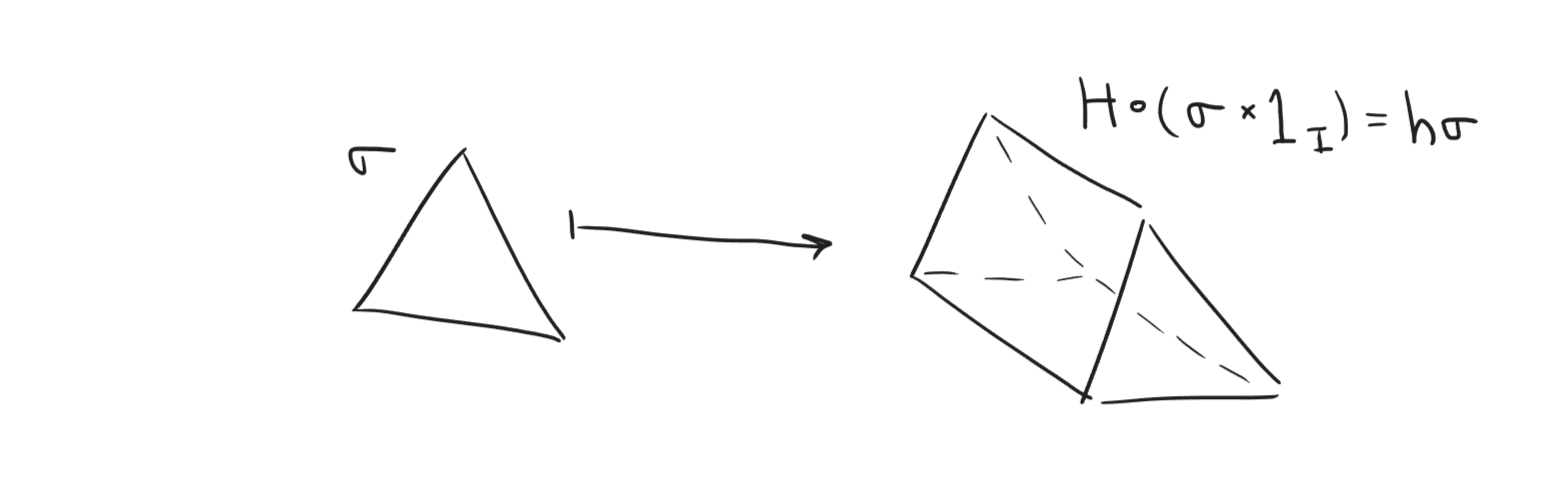
which satisfies \[g_\# - f_\# = \partial h + h \partial.\] Then, we dualize to get a map \[h^*: C^n(Y) \to C^{n-1}(X)\] satisfying \[g^\# - f^\# = h^* \delta + \delta h^*.\] This implies homotopy invariance, since given a cocycle \(\phi \in C^n(Y)\) (i.e., \(\delta \phi=0\)), we get \[g^\#\phi - f^\#\phi = h^* \delta\phi + \delta h^*\phi = \delta h^*\phi,\] so \(g^*[\phi] = f^*[\phi]\) (difference of representative is a coboundary).
Cartan’s Magic Formula
The main insight into the homotopy operator for de Rham cohomology is Cartan’s Magic Formula. It tells you, for a vector field \(X\), that \[\mathcal{L}_X = d\iota_X + \iota_X d.\] We will prove later that \(\mathcal{L}_X: \Omega^*(M) \to \Omega^*(M)\) is a chain map (commutes with \(d\)). Then, in this light, we can interpret the formula as saying that the chain map \(\mathcal{L}_X\) is chain homotopic to the 0 chain map, with chain homotopy \(\iota_X\). In other words, \(\mathcal{L}_X\) is trivial on cohomology.
If we expect de Rham cohomology to be homotopy invariant, then this makes sense—\(\mathcal{L}_X\) is taking the derivative of the flow \(\phi_t\) corresponding to \(X\), and such a flow is a homotopy. So, on the level of cohomology, \([\phi_t^* \omega] = [\omega]\), so taking the derivative of this constant function, we should get \([0]\).
In this way, Cartan’s Magic Formula tells us that \(\iota_X\) is the “infinitesimal” chain homotopy operator, and to get the actual chain homotopy operator, we just need to integrate.
We dedicate this subsection to proving Cartan’s Magic Formula, i.e., that \(\iota_X\) is an infinitesimal homotopy operator, through the formalism of derivations.
Derivations
Definition 3. A graded commutative algebra \(A\) over \(R\) is a graded \(R\)-algebra \[A = \bigoplus_{n=0}^\infty A^i\] such that multiplication satisfies \[a\cdot b = (-1)^{\deg(a)\deg(b)} b\cdot a.\]
Definition 4. A degree \(p\) derivation on \(A\) is a degree \(p\) graded \(R\)-module homomorphism \(d: A\to A\) satisfying the graded Leibniz rule. In other words, \(d\) is \(R\)-linear satisfying
\(d(A^i)\subseteq A^{i+p}\)
\(d(ab) = d(a)b + (-1)^{p\deg(a)}ad(b)\) for \(a\) homogeneous.
Definition 5. A differential graded commutative algebra is a graded commutative algebra \(A\) with a degree \(+1\) derivation \(d\) satisfying \(d^2=0\).
Example 1. The set of all differential forms \[\Omega(M) = \bigoplus_{p=0}^{\infty} \Omega^p(M) = C^\infty(M) \oplus \Omega^1(M) \oplus \cdots \oplus \Omega^n(M)\] with the exterior derivative \(d\) is a differential graded algebra over \(\mathbb{R}\).
Given a vector field \(X\in \Gamma(TM)\), there are also the following natural derivations:
The Lie derivative \(\mathcal{L}_X\) is a degree \(0\) derivation.
The interior derivative \(\iota_X\) is a degree \(-1\) derivation.
Proving these are derivations are lemmas/exercises in Lee.
Recalling that vector fields are derivations, the fact that the Lie bracket is still a derivation is a standard fact. This result generalizes to derivations of higher degrees.
Lemma 1. Let \(A\) be a graded algebra over \(R\), and let \(D_1, D_2\) be graded \(R\)-derivations of degrees \(p_1,p_2\) respectively. Then, \[D = D_1D_2 - (-1)^{p_1 p_2} D_2D_1\] is a derivation of degree \(p_1+p_2\).
Proof. First, \(D\) is clearly a graded \(R\)-module homomorphism of degree \(p_1 + p_2\), since it is the sum of compositions of \(R\)-module homomorphisms with the degrees adding up correctly. It remains to show that \(D\) is a derivation. We compute (analogously to the standard Lie bracket computation) the following expression for \(D_1D_2(ab)\), \[\begin{align*} &= D_1(D_2(a)b + (-1)^{p_2|a|}aD_2(b))\\ &= D_1 D_2(a)b + (-1)^{p_1|a|+p_1p_2} D_2(a)D_1(b) + (-1)^{p_2|a|}D_1(a)D_2(b) + (-1)^{(p_1+p_2)|a|}aD_1D_2(b), \end{align*}\] and swapping the indices we compute the following expression for \(D_2 D_1(ab)\), \[D_2 D_1(a)b + (-1)^{p_2|a|+p_1p_2} D_1(a)D_2(b) + (-1)^{p_1|a|}D_2(a)D_1(b) + (-1)^{(p_1+p_2)|a|}aD_2D_1(b).\] Finally, we get cancellation of the mixed terms by our choice of sign \((-1)^{p_1p_2}\), so indeed \(D\) is a degree \((p_1+p_2)\) \(R\)-derivation. ◻
Cartan’s Magic Formula
First, we prove two lemmas.
Lemma 2. Let \(D\) be a degree \(0\) derivation on \(\Omega(M)\). Let \(p\in M\), and \(b:M\to \mathbb{R}\) a function which is identically 1 on a neighborhood of \(p\). Then, for all \(\omega\in \Omega(M)\), \[D(b\omega)_p = D(\omega)_p.\]
Proof. By definition, \[\begin{align*} D(b\omega) &= D(b)\omega + b D(\omega)\\ &= D(b)\omega + b D(\omega), \end{align*}\] so evaluating at \(p\) we get \[D(b\omega)_p = D(b)_p \omega_p + b(p) D(\omega)_p = 0\omega_p + 1 \cdot D(\omega)_p = D(\omega)_p,\] since a degree \(0\) derivation on \(\Omega(M)\) restricts to a derivation \(D: C^\infty(M) \to C^\infty(M)\) which is just a vector field, which has \(D(b)_p=0\) because \(b\) is constant in a neighborhood of \(p\). ◻
Lemma 3. (Exterior and Lie Derivatives Commute.) Let \(X\) be a vector field and \(\omega\) a differential form. Then, \[\mathcal{L}_X(d\omega) = d(\mathcal{L}_X \omega)\]
Proof. Let \(\theta_t\) be the flow corresponding to \(X\). Then, \[\mathcal{L}_X(d\omega) = \frac{\mathrm d }{\mathrm d t}|_{t=0} (\theta_t)^* d\omega,\] and recalling that the exterior derivative commutes with pullbacks, we get \[\mathcal{L}_X(d\omega) = \frac{\mathrm d }{\mathrm d t}|_{t=0} d (\theta_t)^* \omega = d(\frac{\mathrm d }{\mathrm d t}|_{t=0} (\theta_t)^* \omega),\] (where the exterior derivative commutes with the time derivative by commuting mixed partial derivatives), giving us \[\mathcal{L}_X(d\omega) = d(\mathcal{L}_X \omega).\] ◻
Proposition 1. (Cartan’s Magic Formula.) For \(M\) a smooth manifold, and \(X\) a vector field, \[\mathcal{L}_X = d \iota_X + \iota_X d.\]
Proof. We can recognize the right hand side as \[d \iota_X - (-1)^{\deg(d)\deg(\iota_X)} \iota_X d,\] so it is a graded commutator. Thus, by our lemma, this is a degree 0 derivation (just like \(\mathcal{L}_X\)).
To show that these two derivations agree, we first reduce to a local version of the problem. Given \(\omega \in \Omega(M)\), we need to show that for all \(p\in M\), \[(\mathcal{L}_X \omega)_p = (d\iota_X + \iota_X d)(\omega)_p.\] Choose a chart \(U\) containing \(p\), and choose a bump function \(b\) supported in \(U\) with \(b(p)=1\). Then, for any derivation \(D\), \[D(b\omega)_p = D(\omega)_p.\] Thus, we can assume that \(\omega=b\omega\) is supported in a chart. Let \(x_1,\dots,x_n\) be coordinates for \(U\), so that we can write \[\omega = \sum_I f_I dx_I,\] where \(I\) is an ordered tuple, \(dx_I\) denotes the wedge over \(I\), and each \(f_I \in C^\infty(M)\). In this way, \(\omega\) is in the subalgebra of \(\Omega(M)\) generated by \(0\)-forms and exact \(1\)-forms.
We show \(\mathcal{L}_X\) and \(d\iota_X + \iota_X d\) agree on \(0\)-forms and exact \(1\)-forms, so that they will agree on such \(\omega\) because they are both degree \(0\) derivations.
First, let \(f\in C^\infty(M)\). Then, \[\mathcal{L}_X f = X\cdot f\] and \[(d\iota_X + \iota_X d)(f) = 0 + \iota_Xdf = df(X) = X\cdot f,\] so indeed we get equality.
Next, let \(df \in \Omega^1(M)\) be an exact 1-form. Then, \[\mathcal{L}_X (df) = d(X\cdot f)\] by the lemma, and \[(d\iota_X + \iota_X d)(df) = d(df(X)) + \iota_X(0) = d(X\cdot f),\] so we get equality for exact 1-forms as well. ◻
Integrate Cartan’s Formula
Now that we have Cartan’s Magic Formula, we will get our desired homotopy operator by integration. We first get a homotopy operator for our favorite homotopy—the straight line homotopy.
Theorem 2. Let \(M\) be a \(C^\infty\) manifold, and define the homotopy \[\begin{align*} i_t: M &\longrightarrow M\times I\\ x &\longmapsto (x,t). \end{align*}\] Then, there exists a homotopy operator \(h: \Omega^p(M\times I) \to \Omega^{p-1}(M)\) satisfying \[hd + dh = i_1^* - i_0^*.\]
Proof. We consider \(M\times I \subseteq M\times \mathbb{R}\) as a submanifold. Define a vector field \(S\) on \(M\times \mathbb{R}\) by \[S_{(q,s)} = (0, \frac{\partial }{\partial s}\mid_s)\] (identifying \(T_{(q,s)}M \cong T_q M \times T_s \mathbb{R}\)), so that the corresponding flow composed with the inclusion \(i_0\) gives the homotopy. We have the following picture.
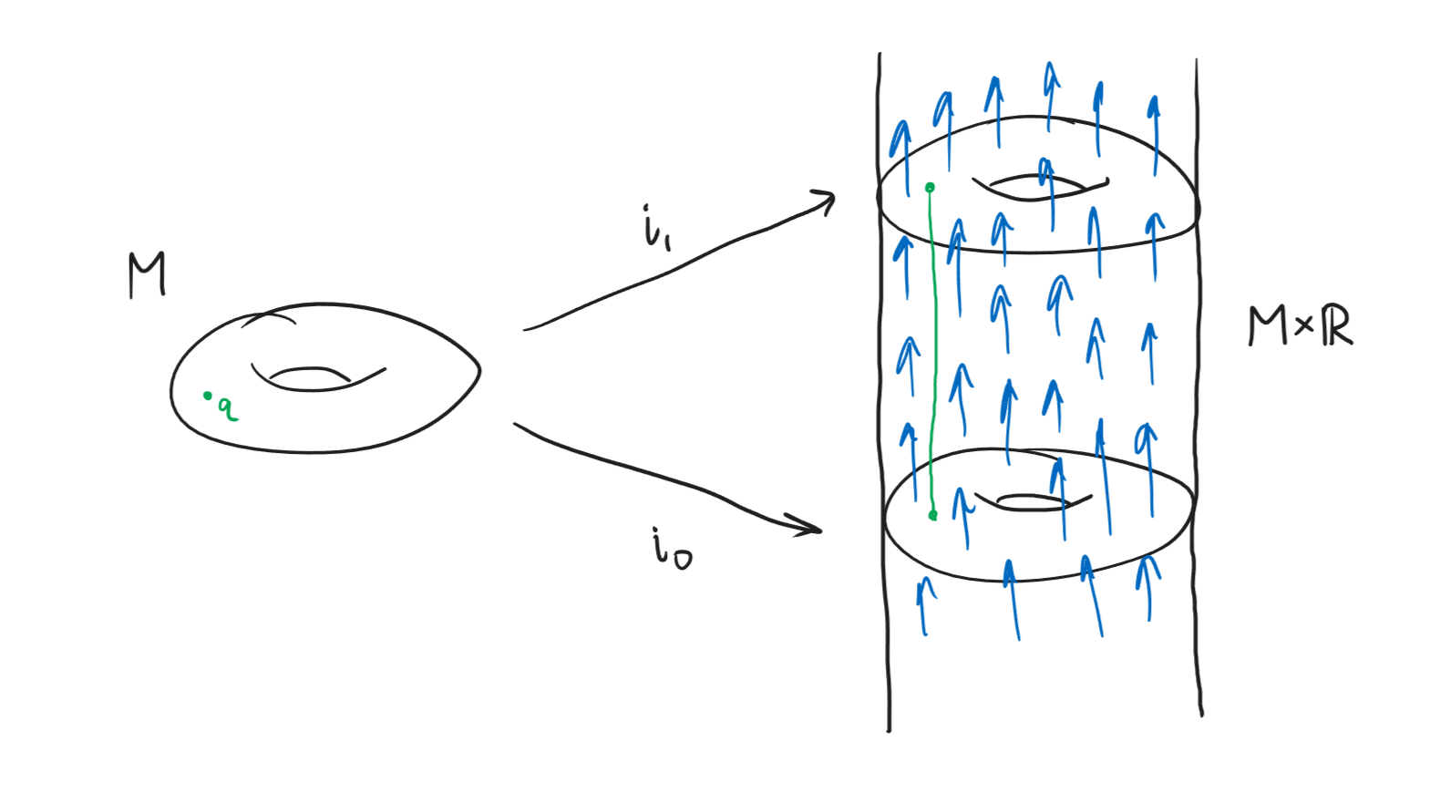
We have a vector field, now we can apply Lie’s Magic Formula. Denoting \(\theta_t\) the flow corresponding to \(S\), and replacing the Lie derivative with its flow definition, Cartan’s formula gives us \[\begin{align*} \frac{\mathrm d }{\mathrm d t}\Big|_{t=0} (\theta_t)^* &= d\iota_S + \iota_S d. \end{align*}\] Precomposing both sides with \(i_t^*\) and using the fact \(i_t = \theta_t \circ i_0\) (from the definition of our vector field), we get \[\begin{align*} (i_t)^* \frac{\mathrm d }{\mathrm d t}\Big|_{t=0} \theta_t^* &= i_t^* d\iota_S + i_t^* \iota_S d\\ \frac{\mathrm d }{\mathrm d t}\Big|_{t=t} i_0^* \theta_t^* &= d i_t^* \iota_S + i_t^* \iota_S d\\ \frac{\mathrm d }{\mathrm d t}\Big|_{t=t} i_t^* &= d i_t^* \iota_S + i_t^* \iota_S d \end{align*}\] and then integrating with respect to \(t\), we have, by the fundamental theorem of calculus \[\begin{align*} i_1^* - i_0^* &= \int_0^1 (d i_t^* \iota_S + i_t^* \iota_S d) dt. \end{align*}\] Now, we can commute the integral with the exterior derivative by differentiating under the integral, to get \[i_1^* - i_0^* = d \int_0^1 (i_t^* \iota_S) dt + \int_0^1 (i_t^* \iota_S d) dt,\] so we should define our homotopy operator \(h:\Omega^p(M\times I) \to \Omega^{p-1}(M)\) by sending \(\omega\in \Omega^p(M\times I)\) \[\omega \longmapsto \int_0^1 (i_t^* \iota_S \omega) dt.\] ◻
Corollary 2. Let \(F,G: M\to N\) be homotopic smooth maps. Then, \(F^*,G^*: H^p(N) \to H^p(M)\) are homotopic.
Proof. Let \(H:M\times I \to N\) be the (not necessarily smooth) homotopy from \(F\) to \(G\). By a corollary of the Whitney approximation theorem, we can assume \(H\) is smooth. Now, we can write the composition

By the previous theorem, \(i_0^* = i_1^*\), so we get \[\begin{align*} i_0^* \circ H^* &= i_1^* \circ H^*\\ (H \circ i_0)^* &= (H \circ i_1)^*\\ F^* &= G^*. \end{align*}\] ◻
Corollary 3 (Homotopy Invariance). If \(M\simeq N\) are homotopy equivalent, then \(H^p(M) \cong H^p(N)\). In particular, if \(M\) is contractible, then \(H^p(M) = H^p(\{\mathrm{pt}\}\)).
Proof. Standard algebraic topology proof. ◻
Finally, to prove the Poincaré Lemma, we compute the de Rham cohomology of a point.
Proposition 2. \(H^0(\{q\}) = \mathbb{R}\) and \(H^p(\{q\}) = 0\) for \(p\geq 1\).
Proof. By definition, \(H^0(\{q\}) = \ker(d: C^\infty(\{q\})\to \Omega^1(\{q\})) / \mathop{\mathrm{im}}0\), which is \(\mathbb{R}\) since the functions on \(\{q\}\) are constant functions \(\mathbb{R}\) which have differential 0. Then, \(H^p(\{q\})=0\) for \(p\geq 1\) since the cohomology groups are quotients of subobjects of \(\Omega^p(\{q\})\), which is 0 already. ◻
Lemma 4 (Poincaré Lemma). If \(M\) is contractible (in particular diffeomorphic to a star-shaped open subset of \(\mathbb{R}^n\) or \(\mathbb{H}^n\)), then \[H^p(M) = \begin{cases} \mathbb{R}& p=0\\ 0 & p\geq 1. \end{cases}\]
Proof. Homotopy invariance + de Rham cohomology of a point. ◻
Commuting with Coboundary
Review of Mayer-Vietoris
Before we can show that the de Rham homomorphism commutes with coboundary (the connecting homomorphism as seen in the Mayer-Vietoris sequence), we review what the coboundary/connecting map even is in both singular and de Rham cohomology.
In de Rham cohomology, we get the Mayer-Vietoris sequence from this SES of chain complexes.

The most convenient thing for us is to see the SES defining Mayer-Vietoris in singular homology, and then to see that the connecting homomorphism for cohomology is calculated using the dual map to that in singular homology (at the level of chains).

where \(C^*(U+V)\) is chain homotopic to \(C^*(M)\) by the inclusion map (reverse direction is barycentric subdivision).
Proving Commutativity
Proposition 3 (Naturality of the de Rham Homomorphism). Let \(M\) be a smooth manifold and \(p\) a nonnegative integer. Then,
If \(F:M\to N\) is a smooth map, then the following diagram commutes:

If \(M\) is a smooth manifold and \(U,V\) are open subsets whose union is \(M\), then the following diagram commutes:

Proof of (a).. This is routine. Let \([\omega]\in H_\mathrm{dR}^p(N)\). To show \(F^*\circ I([\omega]) = I\circ F^*([\omega])\), we show both evaluate the same on smooth simplices. Let \(\sigma\in C_p^\infty(N)\). Then, \[\begin{align*} (I\circ F^*)([\omega])(\sigma) &= I([F^*\omega])(\sigma)\\ &= \int_\sigma F^* \omega\\ &= \int_{\Delta^p} \sigma^*F^*\omega\\ &= \int_{\Delta^p} (F\circ \sigma)^*\omega\\ &= \int_{F\circ \omega} \omega\\ &= (F^*\circ I)([\omega])(\sigma). \end{align*}\] ◻
Proof of (b).. The key is to remember how to compute \(\delta\) and \(\partial^*\), which requires us to remember how the Zig-Zag lemma works and to go back to the SES sequences of chain complexes in de Rham/singular (co)homology which gave us Mayer-Vietoris.
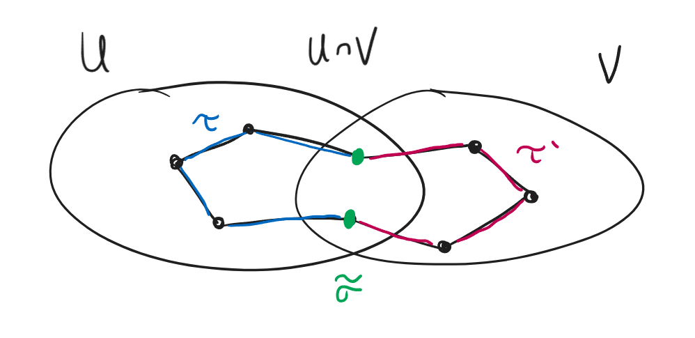
As before, let \([\omega] \in H_\mathrm{dR}^{p-1}(U\cap V)\), and let \([\sigma]\in H_p^\infty(M)\). We will show \[(\partial^* \circ I)([\omega])(\sigma) = (I\circ \delta)([\omega])(\sigma).\] We first compute \((\partial^* \circ I)([\omega])(\sigma)\), using the fact that \(\partial^*\) is really dual to \(\partial_*\) (the connecting homomorphism in homology Mayer-Vietoris), so \[(\partial^* \circ I)([\omega])(\sigma) = I([\omega])(\partial_*\circ \sigma).\] Now, we recall how to compute \(\partial_*\) (going through the Zig-Zag Lemma):
We write \(\sigma = \tau + \tau'\) for some \(\tau\in C_p^\infty(U)\) and \(\tau'\in C_p^\infty(V)\).
We apply boundary to get the pair \((\partial\tau, \partial\tau') \in C_{p-1}^\infty(U)\oplus C_{p-1}^\infty(V)\).
We recognize that \((\partial\tau, \partial\tau')\) come from a chain \(\tilde{\sigma} \in C_{p-1}^\infty(U\cap V)\), i.e., \([\partial\tau]=[\partial\tau']=[\tilde{\sigma}]\)
Therefore, we have \[\begin{align*} (\partial^* \circ I)([\omega])(\sigma) &= I([\omega])(\tilde{\sigma})\\ &= \int_{\tilde{\sigma}} \omega \end{align*}\]
Now, we compute \((I\circ \delta)([\omega])(\sigma)\). By definition of \(\delta\), we do the following.
We choose a preimage of \(\omega\) under \(i_1^* - i_2^*\), say \(\omega = \eta_{U\cap V} - \eta'_{U\cap V}\) for \(\eta\in \Omega^{p-1}(U)\) and \(\eta'\in \Omega^{p-1}(V)\).
Then, we apply the exterior derivative (the coboundary map) to get \(d\eta + d\eta' \in \Omega^p(U)\oplus \Omega^p(V)\).
Finally, it just turns out (i.e., the Zig-Zag lemma proves) that \(d\eta,d\eta'\) comes from a differential form \(\tilde{\omega}\in \Omega^P(M)\).
Then, \(\delta([\omega]) = [\tilde{\eta}]\). Therefore, we have \[\begin{align*} (I\circ \delta)([\omega])(\sigma) &= I([\tilde{\eta}])(\sigma)\\ &=\int_\sigma \tilde{\omega}\\ &=\int_\tau \tilde{\omega} + \int_{\tau'} \tilde{\omega} \tag{$\sigma=\tau+\tau'$}\\ &= \int_\tau d\eta + \int_{\tau'} d\eta' \tag{$\tilde{\omega}$ restricted}\\ &= \int_{\tilde{\sigma}} \eta + \int_{\tilde{\sigma}} \eta' \tag{Stokes' theorem}\\ &= \int_{\tilde{\sigma}} (\eta + \eta')\\ &= \int_{\tilde{\sigma}} \omega \tag{$\omega=\eta+\eta'$} \end{align*}\] ◻
Induction
Our situation is the following: We have two families of functors \(\mathsf{Man}^\infty \to \mathsf{Vec}_\mathbb{R}\) (de Rham cohomology and singular cohomology), and we have a natural transformation \(I\) between them. Both cohomologies give the same answer on contractible spaces, and both cohomologies feature Mayer Vietoris sequences with coboundary commuting with \(I\). It’s our task to argue that \(I\) is an isomorphism for an arbitrary manifold \(M\). The idea is essentially induction—we assume \(I\) is an isomorphism for \(U,V\), then the 5-lemma gets the result for \(U\cup V\).
Theorem 3. For every smooth manifold \(M\) and nonnegative integer \(p\), the de Rham homomorphism \(I: H_\mathrm{dR}^p(M) \to H^p(M;\mathbb{R})\) is an isomorphism.
Proof. In the style of induction, our task is to show for all \(M\), \(I: H_\mathrm{dR}^p(M) \to H^p(M;\mathbb{R})\) is an isomorphism, starting with the “easy” ones.
Terminology. We call a manifold \(M\) de Rham if \(I\) is an isomorphism. We call an open cover \(\{U_i\}\) a de Rham cover if each intersection of \(U_i\) is de Rham. We write \(H^{p-1}(M)\) to be singular cohomology of \(M\) with real coefficients. We call a collection \(\{U_i\}\) a de Rham basis if it is a basis and a de Rham cover.
Strategy. Our base case is convex open subsets. Then, we will show to
Step 1. (Base Case, every convex open subset of \(\mathbb{R}^n\) is de Rham) By the Poincaré lemma, \(H_\mathrm{dR}^p(U)\) is trivial when \(p\neq 0\), which agrees with singular cohomology. We only have to show that \[I: H_\mathrm{dR}^0(U) \to H^0(U;\mathbb{R})\] is an isomorphism, i.e., not the zero map. Let \(f\in \Omega^0(U)\) be a closed form representing a generator \(H_\mathrm{dR}^0(U)\), i.e., a function which is constant (closed on a contractible set) and nonzero. Then, the 0th smooth singular homology of \(U\) is represented by any point \(x\) of \(U\), and \[I([f])([x]) = \int_{x} f = f(x) \neq 0,\] so \(I([f])\neq 0\), so \(I\) is an isomorphism.
Step 2. (Finite Induction, if \(M\) has finite de Rham cover, then \(M\) is de Rham) Suppose \(M=U\cup V\) for \(U,V,U\cap V\) de Rham manifolds. We write down the respective Mayer-Vietoris sequences for both de Rham/singular cohomology, and we write the \(I\) map going down. By the previous section, all of these squares commute, so we have the following commutative diagram with exact rows:

Now, because \(U,V\) are de Rham manifolds, this means every map downwards is an isomorphism, except for potentially the middle map. However, then by the Five Lemma, the middle map is an isomorphism, so \(M\) is a de Rham manifold.
We can use this step repeatedly to show that any \(M\) with a finite de Rham cover is a de Rham manifold.
Step 3. (Infinite-ish Induction, if \(M\) has a de Rham basis, then \(M\) is de Rham) Let \(\{U_i\}\) be a de Rham basis, and let \(f:M\to \mathbb{R}\) be an (any) exhaustion function. For each \(m\in \mathbb{N}\), define \[\begin{align*} A_m &= f^{-1}([m,m+1])\\ A_m' &= f^{-1}((m-\frac{1}{2}, m+\frac{3}{2})). \end{align*}\] so that \(M=\bigcup_{m\in \mathbb{N}} A_m\) is this union of compact sets, and each \(A_m'\) is an open neighborhood of the compact \(A_m\).
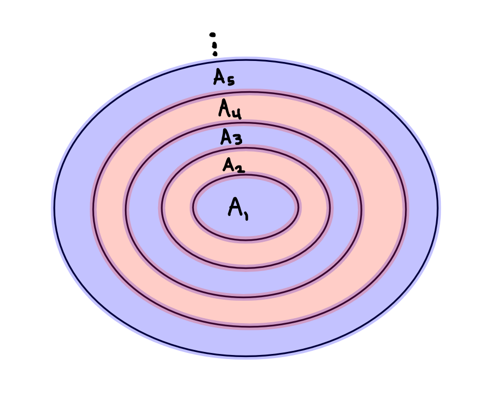
Since \(M\) has a de Rham basis, each point in \(A_m'\) has a de Rham neighborhood, and we can take a finite subcover over \(A_m\) to get a finite de Rham cover of \(A_m\), entirely contained in \(A_m'\). By Step 2, the union of these open sets \(B_m\) is de Rham.
In total, we have these “stripes” of de Rham sets, \(B_1,B_2,B_3,\dots\), and we split the stripes by \[U = B_1 \sqcup B_3 \sqcup \cdots, \qquad V = B_2 \sqcup B_4 \sqcup \cdots,\] where the unions are disjoint because, for example, \(B_1 \subseteq A_1'\) and \(B_3\subseteq A_3'\), but \(A_1'\cap A_3'=\emptyset\).
Now, because the unions are disjoint, and both cohomologies send countable infinite unions to countable infinite direct products in a way commuting with \(I\), we have that \(U,V\) are both de Rham. Furthermore, \(U\cap V\) is de Rham because each intersecting stripe is de Rham (as in the construction of the \(B_m\)), and again it is a countable disjoint union of these stripes.
Thus, by step 2, \(M=U\cup V\) is de Rham.
Step 4. (Apply the Induction) First, any open subset (not necessarily connected!) of \(\mathbb{R}^n\) is de Rham, since it has a basis of open balls which is a de Rham basis. Next, every manifold has a basis of coordinate charts (not necessarily connected!), where each susbset is diffeomorphic to an open subset of \(\mathbb{R}^n\) so is de Rham, and every finite intersection is still a coordinate chart, so still de Rham. This is therefore a de Rham cover, so \(M\) is de Rham. ◻
Remark 1. For a compact manifold, there’s a less technical way of doing this. Choose a metric \(g\) on \(M\), choose a finite open cover of \(M\) by geodesically convex sets \(U_i\). Then, each \(U_i\) is contractible, so we will get \(U_i\) is a de Rham manifold (basically just Poincaré lemma). Furthermore, each intersection is still geodesically convex, so \(\{U_i\}\) forms a finite de Rham cover. Then, the finite induction with the 5-lemma handles the rest.
An Alternative Approach
There’s another approach for proving the de Rham theorem using sheaves, though it is more difficult to see that the isomorphism is exactly given by the de Rham homomorphism, i.e., integration. The proof plays with different ways of computing sheaf cohomology—either Cech cohomology or via an acyclic resolution.
The proof sketch is as follows:
The sheaf cohomology of the constant sheaf \(\underline{\mathbb{R}}\) computes the singular cohomology for \(M\) (and nice spaces in general). This can be seen by choosing a good open cover of \(M\), then computing via Ĉech cohomology that \(H^i(M,\underline{\mathbb{R}})\) is the simplicial cohomology of the nerve of the cover, which is homotopy equivalent to \(M\).
By the Poincaré lemma, the following sequence is exact: \[0\to \underline{\mathbb{R}} \hookrightarrow C^\infty(M) \xrightarrow{d} \Omega^1(M) \to \cdots \xrightarrow{d} \Omega^n(M) \to 0,\] since a surjection in the category sheaves needs only to be locally surjective, i.e., for a closed form \(\omega\) at every point \(p\) there is a contractible neighborhood \(U\) where it is exact, so \(\omega=d\eta\). This means that the sheafification of the image presheaf is exactly the kernel sheaf of the differential.
The differential form sheaves are fine sheaves, i.e., they have partitions of unity. Fine sheaves are acyclic (no higher sheaf cohomology).
Acyclic resolutions compute sheaf cohomology.
Appendix
Random Extra Tools
Exhaustion function. A function \(f:M\to \mathbb{R}\) which has the property that \(f^{-1}((-\infty,c])\) is compact for all \(c\) (called the sublevel sets of \(f\)). These are useful gadgets for generalizing from compact to noncompact manifolds. You can construct them using partitions of unity subordinate to a countable basis of precompact sets.