Representation Theory

Joseph Sullivan

June 2025

Some Definitions/Basics

Always $\mathfrak{g}$ will be a Lie algebra over a field $k$.

Definition. The lower central series of $\mathfrak{g}$ is the sequence of subalgebras defined inductively by \[\mathcal{D}_0 \mathfrak{g}= \mathfrak{g}, \quad \mathcal{D}_k \mathfrak{g}= [\mathfrak{g},\mathcal{D}_{k-1}\mathfrak{g}].\] The derived series of $\mathfrak{g}$ is defined inductively by \[\mathcal{D}^0 \mathfrak{g}= \mathfrak{g}, \quad \mathcal{D}^k \mathfrak{g}= [\mathcal{D}^{k-1} \mathfrak{g}, \mathcal{D}^{k-1} \mathfrak{g}].\] Note that $\mathcal{D}^k \mathfrak{g}\subseteq \mathcal{D}_k \mathfrak{g}$. Also, the Jacobi identity implies that each $\mathcal{D}^k \mathfrak{g}$ is even an ideal.

Definition. We then say that $\mathfrak{g}$ is

abelian if $\mathcal{D}_1 \mathfrak{g}= \mathcal{D}^1 \mathfrak{g}= 0$.
nilpotent if $\mathcal{D}_k \mathfrak{g}= 0$ for $k\gg 0$.
solvable if $\mathcal{D}^k\mathfrak{g}= 0$ for $k\gg 0$.
semisimple if $\mathfrak{g}$ has no nonzero solvable ideals.

Remark. Some easier implications.

Nilpotent implies solvable, since $\mathcal{D}^k \mathfrak{g}\subseteq \mathcal{D}_k \mathfrak{g}$.
The name “solvable” is apt in analogy with group theory, since $\mathcal{D}^k \mathfrak{g}/ \mathcal{D}^{k+1} \mathfrak{g}$ is abelian, since we kill the commutators—so $\mathfrak{g}$ being solvable implies that $\mathfrak{g}$ is filtered by abelian Lie algebras. Even better, the reverse implication also holds.

Abelian Lie algebras are the basic case for representation theory, because of the classic linear algebra fact.

Proposition. Let $A_1,\dots,A_r \in \mathrm{End}(V)$ be commuting operators. Then, they have a common eigenvector in $V$. Assume further that all $A_i$ are diagonalizable, then they are simultaneously diagonalizable.

Now consider a finite dimensional abelian Lie algebra $\mathfrak{h}$ acting diagonally on a vector space, i.e., with a morphism $\mathfrak{h}\to \mathrm{End}(V)$ with each image vector diagonalizable. Then, if $\mathfrak{h}=\left\langle H_i\right\rangle$, the images of each $H_i$ are simultaneously diagonalizable by the proposition, so in fact all of $\mathfrak{h}$ is simultaneously diagonalizable. So, we are able to find spanning vectors $v\in V$ such that \[(\sum a_i H_i) \cdot v = (\sum a_i \lambda_{i,v}) v,\] which is to say that there is a functional $\alpha \in \mathfrak{h}^*$ where \[(\sum a_i H_i)\cdot v = \alpha(\sum a_i H_i) v.\] We will then call $v$ an eigenvector for the $\mathfrak{h}$ action on $V$, and $\alpha$ the eigenvalue of $v$.

Now, we move onto the harder Lie algebras to analyze.

Example. We give some standard examples of nilpotent/solvable/semisimple.

The strictly upper triangular matrices (or any subalgebra) are a nilpotent Lie algebra—$\mathcal{D}_k \mathfrak{g}$ will be matrices with $k$ superdiagonals $0$.
The (not strictly) upper triangular matrices (or any subalgebra) are a solvable Lie algebra.

Proposition. Let $\mathfrak{h}\trianglelefteq \mathfrak{g}$ be an ideal. Then, $\mathfrak{g}$ is solvable iff $\mathfrak{h},\mathfrak{g}/\mathfrak{h}$ are solvable.

In particular, the sum of two solvable ideals $\mathfrak{a}+\mathfrak{b}$ is solvable because \[(\mathfrak{a}+ \mathfrak{b})/\mathfrak{b}\cong \mathfrak{a}/(\mathfrak{a}\cap \mathfrak{b}).\]

Definition. The sum of all solvable ideals is the maximal solvable ideal, called the radical of $\mathfrak{g}$, denoted $\mathrm{rad}(\mathfrak{g})$.

Proposition. $\mathfrak{g}$ is semisimple iff $\mathrm{rad}(\mathfrak{g})=0$.

Corollary. Every Lie algebra fits in an exact sequence \[0 \to \mathrm{rad}(\mathfrak{g}) \to \mathfrak{g}\to \mathfrak{g}/\mathrm{rad}(\mathfrak{g}) \to 0\] where $\mathrm{rad}(\mathfrak{g})$ is solvable and $\mathfrak{g}/\mathrm{rad}(\mathfrak{g})$ is semisimple.

Corollary. $\mathfrak{g}$ is semisimple iff it has no nonzero abelian ideals. As a result, the adjoint representation of a semisimple Lie algebra is faithful (the kernel is the center which is 0).

Definition. Let $\mathfrak{a}$ be a Lie subalgebra of $\mathfrak{g}$. The normalizer of $\mathfrak{a}$ is the Lie subalgebra \[\mathfrak{n}= \{x\in \mathfrak{g}\mid \mathrm{ad}(x)(\mathfrak{a}) \subseteq \mathfrak{a}\}.\]

We finally mention two important theorems for nilpotent/solvable Lie algebras.

Theorem (Engel’s Theorem). A finite dimensional Lie algebra $\mathfrak{g}$ is nilpotent iff for all $X\in \mathfrak{g}$, $\mathrm{ad}X$ is a nilpotent linear operator.

Theorem (Lie’s Theorem). Let $\mathfrak{g}$ be a solvable Lie algebra over $k=\overline{k}$ with $\mathrm{char}(k) = 0$. Then, for $\pi: \mathfrak{g}\to \operatorname{\mathfrak{gl}}(V)$ a finite dimensional representation, there is a complete flag of subrepresentations. That is, $V$ has a basis such that $\mathfrak{g}$ acts by upper triangular matrices.

Representation Theory for $\operatorname{\mathfrak{sl}}_2$

This is essentially the base case to understand the representation theory of general semisimple Lie algebras.

We recall that \[\operatorname{\mathfrak{sl}}_2\mathbb{C}= \{A\in \operatorname{\mathfrak{gl}}(\mathbb{C}^2) \mid \mathrm{tr}A = 0\},\] which has a basis \[H = \begin{bmatrix} 1 & 0\\ 0 & -1 \end{bmatrix}, \quad X = \begin{bmatrix} 0 & 1\\ 0 & 0 \end{bmatrix}, \quad Y = \begin{bmatrix} 0 & 0\\ 1 & 0 \end{bmatrix},\] which have commutators \[[H,X]=2X, \quad [H,Y]=-2Y, \quad [X,Y] = H.\]

Let $V$ be an irreducible finite-dimensional representation of $\operatorname{\mathfrak{sl}}_2\mathbb{C}$. Then, we can study the eigenspaces for the action of $H$ on $V$, \[V_\alpha = \{v\in V \mid H(v) = \alpha\cdot v\}.\] We will eventually see that these encompass all of $V$, i.e., \[V = \bigoplus_\alpha V_\alpha.\] To see this is true, we will show that the right hand side is a subrepresentation. So, we study the action of $X,Y$ on a $V_\alpha$. Let $v\in V_\alpha$, and we want to check that $Xv$ is another eigenvector for $H$, so we compute (using the commutator relations) \[\begin{aligned} HXv &= XHv + [H,X]v\\ &= X\alpha v + 2Xv\\ &= (\alpha+2)Xv, \end{aligned}\] so $Xv$ is indeed an eigenvector for $H$, with eigenvalue $\alpha+2$. Furthermore, we can consider \[X: V_\alpha \to V_{\alpha+2}.\] Analogously, we can compute \[Y: V_\alpha \to V_{\alpha-2}.\] So, fixing an eigenvalue $\alpha$ for $H$, we get that \[\sum_{k\in \mathbb{Z}} V_{\alpha + 2k}\] is a nonzero subrepresentation, so by irreducibility of $V$, all eigenvalues of $H$ differ by even integers, and indeed $V$ is a sum of eigenspaces for $H$.

Since $V$ is finite dimensional, this string of eigenvalues must terminate at either end (the eigenspaces will eventually be zero). Denote $n$ the last eigenvalue (we will later see that this is an integer). We can then draw the $\operatorname{\mathfrak{sl}}_2 \mathbb{C}$ action on $V$ as follows.

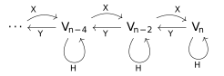
Now, pick $v\in V_n$ nonzero, and we claim the following.

Proposition. $\{v,Yv,Y^2v,\dots\}$ span $V$.

Proof. We check that this span defines a subrepresentation. It is closed under the $Y$ action by construction, and we already know that $H(Y^k v) = (n-2k)v$, so we just need to check the action of $X$. Starting with $v$, we compute \[\begin{aligned} XYv &= [X,Y]v + YXv\\ &= Hv + 0\\ &= nv, \end{aligned}\] and then \[\begin{aligned} XY^k v &= [X,Y]Y^{k-1}v + YXY^{k-1}v\\ &= (n-2(k-1))Y^{k-1}v + Y(XY^{k-1}v), \end{aligned}\] and so induction implies $XY^k v$ is spanned by the $Y^i v$. (Explicitly one can prove \[XY^m(v) = m(n-m+1)Y^{m-1}v\] by more careful induction). ◻

In particular, all eigenspaces $V_\alpha$ of $H$ are one dimensional.

Since $V$ is finite dimensional, there is a smallest power $m$ such that $Y^m v = 0$, which then implies \[0 = XY^m v = m(n-m+1) Y^{m-1}(v),\] so $n=m-1$ is a nonnegative integer, and the eigenvalues of $H$ are just \[n,n-2,\dots,-n+2,-n,\] and the representation is completely determined just by the choice of $n = \dim V - 1$.

One can then realize this representation concretely as $\mathrm{Sym}^n \mathbb{C}^2$.

Representation Theory for General Semisimples

From now on, let $k=\overline{k}$ with $\mathrm{char}(k)=0$, and $\mathfrak{g}$ a semisimple Lie algebra.

Cartan Subalgebra

First, we find the Cartan subalgebra $\mathfrak{h}\subseteq \mathfrak{g}$.

Definition. A Cartan subalgebra is a Lie subalgebra $\mathfrak{h}\subseteq \mathfrak{g}$ such that

$\mathfrak{h}$ is a nilpotent Lie algebra.
$\mathfrak{h}$ is equal to its own normalizer.

We now give a description of how to “find” a Cartan subalgebra from linear algebra concerns. Denote for $h \in \mathfrak{g}, \lambda\in k$ \[\mathfrak{g}(h,\lambda) = \{x\in \mathfrak{g}\mid (\mathrm{ad}h - \lambda I)^p x = 0 \text{ for some } p\in \mathbb{N}\},\] i.e., the generalized eigenspace for $\mathrm{ad}h: \mathfrak{g}\to \mathfrak{g}$ corresponding to eigenvalue $\lambda\in k$. In particular $\lambda=0$ is an eigenvalue since $(\mathrm{ad}h)(h)=0$.

By the Jordan decomposition of $\mathrm{ad}h$, we know \[\mathfrak{g}= \bigoplus_{i=0}^p \mathfrak{g}(h,\lambda_i)\] where $\lambda_0=0,\lambda_1,\dots,\lambda_p$ are the distinct eigenvalues of $\mathrm{ad}h$.

Proposition. Let $h\in \mathfrak{g}$, $\lambda,\mu \in k$, then \[[\mathfrak{g}(h,\lambda),\mathfrak{g}(h,\mu)] \subseteq \mathfrak{g}(h,\lambda + \mu).\] In particular, $\mathfrak{g}(h,0)$ is a Lie subalgebra.

Definition. The rank of $\mathfrak{g}$, denoted $\mathrm{rank}(\mathfrak{g})$, is the smallest algebraic multiplicity for $0$ for $\mathrm{ad}h$ as $h$ ranges in $\mathfrak{g}$.

Proposition. $\mathfrak{g}$ is nilpotent iff $\mathrm{rank}\mathfrak{g}= \dim \mathfrak{g}$.

Proof. Engel’s theorem. ◻

Definition. Call $h\in \mathfrak{g}$ regular if the algebraic multiplicity of $0$ for $\mathrm{ad}h$ achieves the rank.

Remark. Regular elements form a Zariski dense open which are stable under the action of $\mathrm{Aut}(\mathfrak{g})$.

Now, fix a regular element $h_0\in \mathfrak{g}$ and denote \[\mathfrak{h}= \mathfrak{g}(h_0,0).\]

Lemma. The Lie algebra $\mathfrak{h}$ is nilpotent.

Lemma. The Lie algebra $\mathfrak{h}$ is equal to its normalizer.

So, $\mathfrak{h}$ is a Cartan subalgebra. We also have the converse.

Lemma. Let $\mathfrak{h}$ be a Cartan subalgebra of $\mathfrak{g}$. Then, there exists a regular $h\in \mathfrak{g}$ such that $\mathfrak{h}= \mathfrak{g}(h,0)$.

Lemma. $\mathfrak{h}$ is abelian and all $h\in \mathfrak{h}$ are semisimple (i.e., $\mathrm{ad}h$ invariant subspaces have complements, so for $k=\overline{k}$, $\mathrm{ad}h$ is diagonalizable). In particular, $\mathfrak{h}$ is acts diagonally on $\mathfrak{g}$ (commuting diagonalizable operators can be simultaneously diagonalized).

Root Space/Cartan Decomposition

Now, $\mathfrak{h}$ acts on $\mathfrak{g}$ by the adjoint representation, i.e., we have a map \[\mathfrak{h}\xrightarrow{\mathrm{ad}} \operatorname{\mathfrak{gl}}(\mathfrak{g}).\] When we simultaneously diagonalize this action, we get something like a direct sum of eigenspaces, but the eigenvalues will vary from operator to operator—this varying is tracked by a functional on $\mathfrak{h}$. Indeed, if $X\in \mathfrak{g}$ is a simultaneous eigenvector not in $\mathfrak{h}$ ($\mathfrak{h}$ acts trivially on $\mathfrak{h}$ so this isn’t interesting), then the assignment

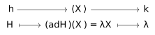
is linear, so we can define this to be a functional $\alpha\in \mathfrak{h}^*$. We call $\alpha$ (nonzero) a root of the Lie algebra, and we define \[\mathfrak{g}_\alpha = \{X\in \mathfrak{g}\mid (\mathrm{ad}H)X = \alpha(H)\cdot X \text{ for all } H\in \mathfrak{h}\}\] the root space. Then, our “eigenspace” decomposition of $\mathfrak{g}$, called the root space/Cartan decomposition is \[\mathfrak{g}= \mathfrak{h}\oplus (\bigoplus_{0\neq \alpha \in \mathfrak{h}^*} \mathfrak{g}_\alpha).\] Denote the $\alpha\neq 0$ such that $\mathfrak{g}_\alpha\neq 0$ by $R$, i.e., the set of roots.

Proposition. Properties of root spaces.

Each root space $\mathfrak{g}_\alpha$ is one dimensional.
$R$ generates a lattice $\Lambda_R \subseteq \mathfrak{h}^*$ called the root lattice of rank equal to the dimension of $\mathfrak{h}$.
$R$ is symmetric about the origin, i.e., if $\alpha\in R$, then $-\alpha \in R$.

In light of the root space decomposition, we can start analyzing representations of $\mathfrak{g}$. Say $\mathfrak{g}\xrightarrow{\sigma} \operatorname{\mathfrak{gl}}(V)$ is an irreducible finite dimensional representation of $\mathfrak{g}$. Define for a functional (not necessarily a root) $\alpha\in \mathfrak{h}^*$ \[V_\alpha = \{v\in V \mid \forall H\in \mathfrak{h}, H\cdot v = \alpha(H)(v)\}\] which, if nonzero, we call a weight space for $V$, and $\alpha$ a weight. We call the dimension of $V_\alpha$ the multiplicity of the weight $\alpha$.

We claim that \[\bigoplus V_\alpha = V.\] To see this, we note that the left hand side is nonzero, since $k=\overline{k}$ means we can find an eigenvector for the commuting family $\sigma(\mathfrak{h})$. Then, we show that the left hand side is actually a nontrivial $\mathfrak{g}$-submodule, so by irreducibility it is all of $V$.

To check that this is a $\mathfrak{g}$-submodule, we check the $\mathfrak{g}$ action by studying each component in the root space decomposition. First, by definition of the weight spaces, $\mathfrak{h}\cdot V_\alpha \subseteq V_\alpha$. Now, we check the action of $\mathfrak{g}_\beta$. We claim \[\mathfrak{g}_\beta \cdot V_\alpha \subseteq V_{\alpha+\beta},\] and indeed if $X\in \mathfrak{g}_\beta$ and $v\in V_\alpha$, then for any $H\in \mathfrak{h}$ \[\begin{aligned} \sigma(H)\sigma(X)v &= \sigma(X)\sigma(H)v + \sigma([H,X])v\\ &= \sigma(X)\alpha(H)v + \sigma((\mathrm{ad}H)X)v\\ &= \alpha(H)\sigma(X)v + \sigma(\beta(H)X)v\\ &= (\alpha + \beta)(H)\sigma(X)v. \end{aligned}\]

This also tells us that the weights live in a translate of the root lattice, since fixing a weight $\alpha$ and considering \[\sum_{\beta\in R} V_{\alpha+\beta}\] we would get a nonzero subrepresentation, but again we are assuming $V$ is irreducible.

Many $\operatorname{\mathfrak{sl}}_2\mathbb{C}$ Representations

We find distinguished subalgebras $\mathfrak{s}_\alpha \cong \operatorname{\mathfrak{sl}}_2 \mathbb{C}\subseteq \mathfrak{g}$.

Before, we stated each root space $\mathfrak{g}_\alpha$ is one dimensional, as is $\mathfrak{g}_{-\alpha}$, and we note \[[\mathfrak{g}_\alpha,\mathfrak{g}_{-\alpha}] \subseteq \mathfrak{h}\] spans at most one dimension, giving us a subalgebra \[\mathfrak{s}_\alpha = \mathfrak{g}_\alpha \oplus \mathfrak{g}_{-\alpha} \oplus [\mathfrak{g}_\alpha, \mathfrak{g}_{-\alpha}].\]

Proposition. Commutator facts.

$[\mathfrak{g}_\alpha,\mathfrak{g}_{-\alpha}] \neq 0$
$[[\mathfrak{g}_\alpha,\mathfrak{g}_{-\alpha}],\mathfrak{g}_\alpha] \neq 0$

and consequently $\mathfrak{s}_\alpha \cong \operatorname{\mathfrak{sl}}_2\mathbb{C}$.

We then pick out a basis $X_\alpha\in \mathfrak{g}_\alpha, Y_\alpha\in \mathfrak{g}_{-\alpha}, H_\alpha \in [\mathfrak{g}_\alpha,\mathfrak{g}_{-\alpha}]$ satisfying the commutation relations for $\operatorname{\mathfrak{sl}}_2\mathbb{C}$.

Note that $H_\alpha\in [\mathfrak{g}_\alpha,\mathfrak{g}_{-\alpha}]$ is uniquely determined by having eigenvalues $2$ and $-2$ on $\mathfrak{g}_\alpha,\mathfrak{g}_{-\alpha}$ respectively.

(Just for my sanity, note that \[2X_\alpha = [H_\alpha,X_\alpha] = (\mathrm{ad}H_\alpha)(X_\alpha)=\alpha(H_\alpha)X_\alpha,\] so $\alpha(H_\alpha)=2$, and we should think of the weight $\alpha$ as an even integer for the adjoint representation).

Integrality of Eigenvalues

By our analysis of $\operatorname{\mathfrak{sl}}_2\mathbb{C}$, we know that our induced representation from $\mathfrak{g}$ will be such that the action of $H_\alpha$ has only integer eigenvalues. This means that every weight $\beta\in \mathfrak{h}^*$ of a representation of $\mathfrak{g}$ must assume integer values on all the $H_\alpha\in \mathfrak{h}$, since taking $v \in V_\beta$ nonzero, we get \[H_\alpha \cdot v = \beta(H_\alpha)\cdot v,\] so in particular $\beta(H_\alpha)$ is an eigenvalue of $H_\alpha$ under a representation.

Let $\Lambda_W$, which we call the weight lattice, be the set of linear functionals $\beta \in \mathfrak{h}^*$ that are integer valued on all the $H_\alpha$. Our analysis shows that all weights of a representation of $\mathfrak{g}$ lie in $\Lambda_W$. In particular, $R,\Lambda_R \subseteq \Lambda_W$.

Use Symmetry to Find Eigenvalues of $H_\alpha$

We define $W_\alpha$ to following involution on $\mathfrak{h}^*$. Define \[\Omega_\alpha = \{\beta\in \mathfrak{h}^* \mid \beta(H_\alpha)=0\},\] and set $W_\alpha$ to be the reflection in this plane spanned by $\alpha$, so \[W_\alpha(\beta) = \beta - \frac{2\beta(H_\alpha)}{\alpha(H_\alpha)} = \beta - \beta(H_\alpha)\alpha.\] Let $\mathcal{W}$ be the group generated by these involutions, called the Weyl group.

(Note that on a semisimple Lie algebra the Killing form $B(X,Y):=\mathrm{tr}(\mathrm{ad}X \circ \mathrm{ad}Y)$ is an inner product, which gives an identification $\mathfrak{h}\cong \mathfrak{h}^*$. We claim this sends $H_\alpha \mapsto \alpha$, so we need to check for all $H\in \mathfrak{h}$ $B(H_\alpha,H)=\alpha(H)$ how to check??? is this true???)

Now, suppose $V$ is a weight module for $\mathfrak{g}$, and we partition the weight spaces into $\alpha$ cosets, and then the weights spaces of a coset \[V_{[\beta]} = \bigoplus_{n\in \mathbb{Z}} V_{\beta+n\alpha}\] will be a subrepresentation of $V$ for $\mathfrak{s}_\alpha$ (just check the action of $X_\alpha,Y_\alpha,H_\alpha$), and we know that the weights appearing in a subrepresentation are symmetric about 0, which implies that the weights are invariant under the Weyl group.

Choosing a Direction

Pick a real linear functional $\ell: \Lambda_R \to \mathbb{R}$ irrational with respect to the lattice ( not sending any nonzero points to 0???). This gives a decomposition \[R = R^+ \cup R^-\] by $R^+ = \{\alpha \mid \ell(\alpha)>0\}$ and vice versa, which is called an ordering of the roots.

Definition. Let $V$ be a representation of $\mathfrak{g}$. A nonzero vector $v\in V$ that is both an eigenvector for the action of $\mathfrak{h}$ (in a weight space) and in the kernel of a $\mathfrak{g}_\alpha$ for all $\alpha \in R^+$ is called a highest weight vector of $V$. The weight $\alpha$ such that $v\in V_\alpha$ is called the highest weight.

From now on, $\alpha$ will denote the highest weight $V$ for our ordering.

Proposition. Properties of highest weight vectors.

Every finite-dimensional representation $V$ of $\mathfrak{g}$ possesses a highest weight vector.
The subspace $W$ of $V$ generated by the images of a highest weight vector $v$ under successive applications of root spaces $\mathfrak{g}_\beta$ for $\beta \in R^-$ is an irreducible subrepresentation.
An irreducible representation possesses a unique highest weight vector up to scalars (i.e., $\mathfrak{g}_\alpha$ is 1-dimensional).

In fact, we don’t even need to use all $\beta\in R^-$ to generate a subrepresentation, we just need to use semigroup generators. We call a positive (resp. negative) $\alpha\in R$ primitive or simple if it cannot be expressed as a sum of two positive (resp. negative) roots. These serve as semigroup generators (by finiteness of $R$).

So, we have a highest weight vector, but we still need to describe the remaining vectors. The point is that choosing the ordering of the roots gave us a “farthest” direction, which is the highest weight. However, there should be symmetry, that we could have easily chosen a different ordering, and this should affect the story. More concretely, we have the following fact.

Proposition. Every vertex of the convex hull of the weights of $V$ must be conjugate to $\alpha$ under the Weyl group.

Proposition. The weights of $V$ will be exactly the weights that are congruent to $\alpha$ modulo the root lattice $\Lambda_R$ and that lie in the convex hull of the images of $\alpha$ under the Weyl group, i.e., \[\mathrm{Conv}(\mathcal{W}\cdot \alpha) \cap (\Lambda_R + \alpha).\]

When it comes to finding irreps of $\mathfrak{g}$, we will be choosing a highest weight $\alpha$ for $R^+$, which will need to satisfy $\alpha(H_\gamma)\geq 0$ for every $\gamma\in R^+$. We then give a name for the set of $\alpha$ satisfying this condition.

Definition. The (closed) Weyl chamber associated to the ordering of the roots is the set $\mathfrak{W}\subseteq \mathbb{R}\cdot R$ defined by \[\mathfrak{W}= \{\alpha\in \mathbb{R}\cdot R \mid \alpha(H_\gamma)\geq 0 \text{ for all } \gamma \in R^+\}.\]

If we identify $\gamma$ and $H_\gamma$ by the killing form, this condition expresses that $\alpha$ is “aligned” towards all $\gamma$, that the angle between $\gamma,\alpha$ is at most a right angle.

The Weyl group acts transitively on the orderings of the roots, and hence also the Weyl chambers.

Classifying Representations

Theorem. For any $\alpha$ in the intersection of the weight lattice $\Lambda_W$ and the Weyl chamber $\mathfrak{W}$ (associated to the ordering of the roots), there exists a unique irreducible finite dimensional representation $\Gamma_\alpha$ of $\mathfrak{g}$ with highest weight $\alpha$. This gives a bijection between $\mathfrak{W}\cap \Lambda_W$ and the irreps of $\mathfrak{g}$. The weights of $\Gamma_\alpha$ consists of those elements of $\Lambda_W$ congruent to $\alpha$ modulo $\Gamma_R$ lying in the convex hull of points in $\mathfrak{h}^*$ conjugate to $\alpha$ under the Weyl group.

There also exist fundamental weights $\omega_1,\dots,\omega_n$ with the property that any highest weight can be expressed as a unique nonnegative integral linear combination of them. Geometrically, these are the first weights met along the edges of a Weyl chamber. Algebraically, these satisfying \[\left\langle\omega_i,\alpha_j\right\rangle = \delta_{ij}\] where $\alpha_1,\dots,\alpha_n$ are the simple roots.

Then, we will write for $a_1,\dots,a_n\in \mathbb{Z}_{\geq 0}$ an irrep by \[\Gamma_{a_1,\dots,a_n} = \Gamma_{a_1\omega_1+\dots+a_n\omega_n}.\]

Borel-Weil-Bott

Let $G$ be a semisimple Lie group with Lie algebra $\mathfrak{g}$ and Cartan subalgebra $\mathfrak{h}$. The Cartan subalgebra exponentiates to a closed subgroup $H\leq G$ which is a maximal torus. We then have a root space decomposition \[\mathfrak{g}= \mathfrak{h}\oplus \bigoplus_{\alpha\in R} \mathfrak{g}_\alpha.\] Choose an ordering of the roots \[R = R^+ \sqcup R^-.\]

Definition. The Borel subalgebra is the subalgebra \[\mathfrak{b}= \mathfrak{h}\oplus \bigoplus_{\alpha\in R^+} \mathfrak{g}_\alpha.\] The connected closed subgroup $B$ of $G$ with Lie algebra $\mathfrak{b}$ is called the Borel subgroup.

Remark. $B$ is closed because it can be realized as the preimage under \[G \xrightarrow{\mathrm{ad}} \mathrm{GL}(\mathfrak{g})\] of the subgroup of $\mathrm{GL}(\mathfrak{g})$ that preserves $\mathfrak{b}$.

Let $\lambda\in \Lambda_W$ be a weight. Then, $\lambda$ exponentiates to a homomorphism $e^\lambda: H\to \mathbb{C}^*$ ( why? because $\Lambda_W\subseteq \mathfrak{h}^*$ full rank lattice will be sent to $1$ under exponential map?). We can extend this trivially to $B\to \mathbb{C}^*$, since $B$ is a semidirect product of $H$ and the nilpotent subgroup $N$ with Lie algebra a direct sum of just the $\mathfrak{g}_\alpha$ for $\alpha\in R^+$ (notice that $N$ is normal, the product of $N,H$ is all of $B$, and $N\cap H=\{e\}$). So, every $x\in B$ is of the form $nh$, and so we send $nh\mapsto e^{\lambda}(h)$. ( alternatively, I think it’s just true that $N=[B,B]$ and $H\cong B/[B,B]$, so not really any different, but we’re just precomposing $e^\lambda$ with the projection).

Denote this representation $B\to \mathrm{GL}_1(\mathbb{C})$ by $\mathbb{C}_\lambda$.

Now, we can define a line bundle \[\begin{aligned} L_\lambda &= G\times_B \mathbb{C}_\lambda\\ &= (G\times \mathbb{C}_\lambda)/\{(g,xv) \sim (gx,v), x\in B\}, \end{aligned}\] with its natural projection to $G/B$. This will be a holomorphic line bundle, and Borel-Weil-Bott predicts its cohomology.

Denote $\rho = \frac{1}{2}\sum_{\alpha\in R^+} \alpha$, and denote the Weyl group action centered at $-\rho$ by which for $w\in \mathcal{W}$, $\lambda\in \Lambda_W$ \[w*\lambda :=w(\lambda+\rho) - \rho.\]

Call a weight $\lambda$ dominant if it is in the closed Weyl chamber.

Define the length function $\ell: \mathfrak{W}\to \mathbb{N}$ as follows. For our ordering of $R$, we have standard generators of $\mathcal{W}$ which are reflections $W_\alpha$ about the simple roots $\alpha$. Now, for an arbitrary $w\in \mathcal{W}$, define its length $\ell(w)$ the length of the shortest word defining $w$ using the standard generators.

Theorem. Let $\lambda$ be an integral weight. Then, we have two cases.

There is no $w\in \mathcal{W}$ such that $w*\lambda$ is dominant. Then, \[H^i(G/B,L_\lambda) = 0 \quad \text{for all $i$}.\]
There is a unique $w\in \mathcal{W}$ such that $w*\lambda$ is dominant. Then, \[H^i(G/B,L_\lambda) = \begin{cases} 0 & i\neq \ell(w)\\ (\Gamma_{w*\lambda})^\vee & i=\ell(w). \end{cases}\]

Remark. Recall if $V$ is a representation of $G$, we get a dual representation $V^\vee = \mathrm{Hom}_\mathbb{C}(V,\mathbb{C})$ by \[g\cdot f(-) = f(g^{-1}\cdot (-)),\] or more concretely, when $V=\mathbb{C}^n$, and our original representation is \[\rho: G\to \mathrm{GL}(V),\] this is \[g \mapsto (\rho(g)^{-1})^T.\]

Now, for a Lie algebra representation $V$ of $\mathfrak{g}$, the dual representation is given by \[X\cdot f(-) \mapsto -f(X(-)).\]

One can see from this description that the weights of $V^\vee$ are exactly the negations of the weights of $V$, so the highest weight is the negation of the “lowest weight”, which occurs in the negative Weyl chamber. There is a unique element $w_0\in \mathfrak{W}$ that maps the negative Weyl chamber to the Weyl chamber, so we get that the highest weight of $V^\vee$ is \[w_0 \cdot (-\lambda),\] where $\lambda$ is the highest weight of $V$.

Representation Theory of $\operatorname{\mathfrak{sl}}_n \mathbb{C}$

Let $V=\mathbb{C}^n = \left\langle x_1,\dots,x_n\right\rangle$. We will carry some of the representation theory program through for $\operatorname{\mathfrak{sl}}_n \mathbb{C}= \operatorname{\mathfrak{sl}}V$, and then understand the Borel-Weil-Bott theorem for the representations $\mathrm{Sym}^m V$.

First, we recall \[\operatorname{\mathfrak{sl}}V = \{A\in \operatorname{\mathfrak{gl}}V \mid \mathrm{tr}A = 0\},\] i.e., the traceless matrices on $V$. A suitable Cartan subalgebra is the subalgebra of diagonal matrices \[\mathfrak{h}= \{\sum a_i H_i \mid \sum a_i = 0\},\] where $H_i=E_{i,i}: V\to V$ is the operator sending $x_i\mapsto x_i$ and $x_j\mapsto 0$.

On the ambient space of all diagonal matrices, the $H_i$ give a basis, so we get a dual basis $L_i$ by $L_i(H_j)=\delta_{ij}$. The restriction of the $L_i$ to $\mathfrak{h}$ then gives a generator set for $\mathfrak{h}^*$. Finding the relations, we can write \[\mathfrak{h}^* = \mathbb{C}\{L_i\}/(\sum L_i).\]

Now, we find the root space decomposition with respect to this Cartan subalgebra. So, we need to find the “eigenvectors” for the adjoint action. We already know how $\mathfrak{h}$ acts on $\mathfrak{h}$ itself—this is the 0 map, since $\mathfrak{h}$ is abelian. Now, to see the remainder of the action, we should compute the action of $\mathfrak{h}$ on an off diagonal $E_{i,j}$ (i.e., $i\neq j$).

We compute \[\mathrm{ad}(\sum a_i H_i) E_{i,j} = (a_i - a_j)E_{i,j} = (L_i - L_j)(\sum a_i H_i) E_{i,j},\] so in fact each of the usual basis vectors $E_{i,j}$ are eigenvectors for our action, and our roots are exactly \[R =\{ L_i - L_j \in \mathfrak{h}^* \mid i\neq j \}.\]

We can then pick out the $\operatorname{\mathfrak{sl}}_2 \mathbb{C}$ representations $\mathfrak{s}_{L_i-L_j}$ by picking \[X_{L_i - L_j} = E_{i,j}, \quad Y_{L_i - L_j} = E_{j,i}, \quad H_{L_i - L_j} = [E_{i,j},E_{j,i}] = H_i - H_j,\] (check the commutators).

With $H_{L_i-L_j}$ we can compute the weight lattice as the integer valued functions. These are spanned by the $L_i$, so \[\Lambda_W = \mathbb{Z}\{L_i\}/(\sum L_i),\] whereas the root lattice is \[\Lambda_R = \mathbb{Z}\{L_i - L_j\}.\]

For fun, we can observe that $\Lambda_W / \Lambda_R$ is generated by any $L_i$ (the remaining $L_j$ can be gotten by adding $L_j - L_i$), so the abelian group is cyclic. In fact, $nL_i \in \Lambda_R$, since we can write \[nL_i = \sum_i (L_i - L_j) + \sum_j L_j,\] and even more, no earlier $kL_i \in \Lambda_R$ ( some sort of geometry argument... argue that the $L_i-L_j$ are the smallest norm vectors in $\Lambda_R$, and nonzero sums of 2 of these are strictly bigger??), so $\Lambda_W/\Lambda_R=\mathbb{Z}/n\mathbb{Z}$.

Now, to describe the irreducible representations, we choose a direction and describe the Weyl chamber. To choose an irrational linear function $\ell$ on $\Lambda_W$, we need to images $c_i$ for each $L_i$ satisfying $\sum c_i = 0$. To be irrational, we just need to choose for example $c_1>c_2>\cdots>c_n$, which then gives the ordering of the roots \[R^+ = \{L_i - L_j \mid i< j\}, \quad R^- = \{L_i - L_j \mid j <i\}.\] The primitive roots are then $L_{i+1}-L_i$. The (closed) Weyl chamber is then \[\mathfrak{W}= \{\sum a_i L_i \mid a_1\geq a_2\geq \cdots \geq a_n\},\] whose rays are generated by \[L_1, L_1 + L_2, \cdots, L_1+\cdots+L_{n-1} = -L_n,\] which are the smallest elements of $\Lambda_W$ along the rays, so these are the fundamental weights, \[\omega_i = L_1 + \cdots + L_i,\] which gives us a parameterization of the irreps of $\operatorname{\mathfrak{sl}}_n \mathbb{C}$ by $\Gamma_{a_1,\dots,a_{n-1}}$.

Proposition. $\bigwedge^i V$ is an irrep of highest weight $\omega_i$.

Proof. For \[J = \{j_1<j_2<\cdots<j_i\} \subseteq \{1,\dots,n\}\] a cardinality $i$ subset, denote \[e_J = e_{j_1}\wedge \cdots \wedge e_{j_i}.\] As we vary $J$, we get a basis for $\bigwedge^i V$, and we observe that \[(\sum a_i H_i)\cdot e_J = (\sum_{i\in J} a_i) \cdot e_J = (\sum_{i\in J} L_i)(\sum a_i H_i)e_J,\] so $e_J$ is a weight vector of weight $\sum_{i\in J} L_i$. In particular, this proves that $\bigwedge^i V$ is irreducible, since it is a sum of weight spaces all of dimension 1, whose weights are all congruent $\Lambda_R$.

Now, to maximize our direction, we should take $J=\{1,\dots,i\}$, so the highest weight is \[L_1+\cdots+L_i = \omega_i.\] ◻

Corollary. The irrep $\Gamma_{a_1,\dots,a_{n-1}}$ is a subrepresentation of \[\mathrm{Sym}^{a_1} \bigwedge^1 V \otimes \mathrm{Sym}^{a_2}\bigwedge^2 V \otimes \cdots \otimes \mathrm{Sym}^{a_{n-1}}\bigwedge^{n-1} V.\]

Proof. Notice that \[(e_1)^{a_1} \otimes (e_1 \wedge e_2)^{a_2} \otimes \cdots \otimes (e_1\wedge \cdots \wedge e_{n-1})^{a_{n-1}}\] is a weight vector, with weight \[a_1 \omega_1 + \cdots + a_{n-1} \omega_{n-1}\] (just check the action of $\sum b_i H_i$). The $\operatorname{\mathfrak{sl}}_n \mathbb{C}$ span of this vector will then be $\Gamma_{a_1,\dots,a_{n-1}}$. ◻

In this sense we have found all of the irreps, by looking at the $\operatorname{\mathfrak{sl}}_n \mathbb{C}$ spans of weight vectors inside these representations.

Flag Variety

From our choice of Cartan subalgebra and direction, the Borel subgroup is the lower triangular matrices of $\mathrm{SL}V$. To see this, note that corresponding to a positive root $L_i-L_j$ for $i>j$, we get generator $X_{L_i-L_j}=E_{i,j} \in \mathfrak{g}_{L_i-L_j}$. So, the Borel subalgebra is given by \[\mathfrak{h}\oplus \sum_{\alpha\in R^+} = \mathfrak{h}\oplus \sum_{i>j} \mathbb{C}\cdot E_{i,j},\] which exponentiates to the lower triangular matrices $\mathrm{SL}V$.

Now, $G/B$ actually has the structure of an algebraic variety, and is the complete flag variety $\mathrm{Fl}(V)$. As a set \[\mathrm{Fl}(V) :=\{0=\ell_0 < \ell_1 < \cdots < \ell_{n-1} < \ell_n=V\},\] the set of maximal sequences of vector subspaces in $V$, which are called flags. Like projective space and Grassmannians, these are varieties. One way to give $\mathrm{Fl}(V)$ the structure of a variety is to recognize it as a closed subset inside a product of Grassmannians \[\mathrm{Fl}(V) \subseteq \mathrm{Gr}(1,V) \times \mathrm{Gr}(2,V) \times \cdots \times \mathrm{Gr}(n-1,V),\] where $\mathrm{Fl}(V)$ is cut out by the incidence correspondence, i.e., the relation that $\ell_i \in \mathrm{Gr}(i,V)$ is a subspace of $\ell_{i+1} \in \mathrm{Gr}(i+1,V)$. To see this as a closed subset, we can either work locally in charts (think Plücker coordinates, checking ) even recognize this as the vanishing of a section of a vector bundle

Applying Borel-Weil-Bott

Let’s try to find bundles with prescribed cohomology on $\mathbb{P}V$ using Borel-Weil-Bott. In particular, we will try to “find” $\mathcal{O}_{\mathbb{P}V}(a)$ knowing that its global sections is $\mathrm{Sym}^a V^\vee$.

We will be constructing bundles $L_\lambda$ on $G/B$, which is the complete flag variety in $V$. We then have a projection $G/B \xrightarrow{\pi} \mathbb{P}V$, so we will hope to get our bundles by studying pushforwards $\pi_* L_\lambda$.

If we want cohomology $\mathrm{Sym}^a V^\vee$, we should first find $\lambda$ such that $\Gamma_\lambda^\vee \cong \mathrm{Sym}^a V^\vee$, so $\lambda$ will be the negation of the lowest weight of $\mathrm{Sym}^a V^\vee$, i.e., the highest weight of the dual.

Then, one can compute that $\mathrm{Sym}^a V$ is the dual representation of $\mathrm{Sym}^a V^\vee$ (either directly or by analyzing lowest/highest weights) to get our choice $\lambda = aL_1$. Now, we get an induced map \[\begin{aligned} e^\lambda: B &\longrightarrow \mathrm{GL}_1(\mathbb{C})\\ b &\longmapsto (z \mapsto b_{11}^a \cdot z), \end{aligned}\] which we can check is correct by differentiating.

So, as per Borel-Weil-Bott, we construct $L_\lambda$. which has total space \[G\times_B \mathbb{C}_\lambda = \{(g,z)\}/(gb,z) \sim (g,bz).\]

How will we recognize this bundle? Maybe realize $G/B$ as a closed subvariety of a product of Grassmannians, so we can ask if $L_\lambda$ is a pullback from \[\mathbb{P}V \times \mathrm{Gr}(2,V) \times \cdots \times \mathrm{Gr}(n-1,V),\] and then try to pushforward from here?

Representation Theory of $\mathfrak{so}(Q)$

Structure of Quadratic Forms

Let $k$ be a field, let $W$ be a vector space with basis $x_1,\dots,x_n$, and let \[Q\in \mathrm{Sym}^2 W = k[x_1,\dots,x_n]_2\] be a quadratic form.

Proposition. $Q$ can be diagonalized, i.e., there exists a linear change of coordinates $T:W\to W$ such that \[\mathrm{Sym}^2(T)(Q) = a_1 x_1^2 + \dots + a_n x_n^2\] for some $a_i\in k$.

Proof. We prove the proposition by induction on the smallest $m\in \mathbb{N}$ such that \[Q\in k[x_1,\dots,x_m]_2 \hookrightarrow k[x_1,\dots,x_n]_2.\] If $m=0,1$, then we are done.

Otherwise, assume $m>1$. Our strategy is to change coordinates to write \[Q = a_m x_m^2 + Q'\] with $Q'\in k[x_1,\dots,x_{m-1}]_2$, and then finish by our induction hypothesis. So, we need to “get rid” of any $x_m x_i$ cross-terms by changing our $x_m$ coordinate.

First, however, we need a nonzero $a x_m^2$ term (in case we only have cross-terms). If $a=0$, by definition of $m$, we can at least pick a nonzero term \[c x_m x_i\] of $Q$, and change coordinates by sending $x_i \mapsto x_m+x_i$, so that our $x_m^2$ coefficient becomes $c\neq 0$.

Now, we our quadratic form looks like \[Q = a \left(x_m^2 + \sum_{i=1}^{m-1} \frac{b_i}{a} x_m x_i\right) + Q'\] for some $Q'\in k[x_1,\dots,x_{m-1}]_2$. We can then rewrite $Q-Q'$ as \[a\left(x_m + \sum_{i=1}^{m-1} \frac{b_i}{2a} x_i\right) + \text{term in $k[x_1,\dots,x_{m-1}]_2$},\] so if we change coordinates by \[x_m \mapsto x_m - \sum_{i=1}^{m-1} \frac{b_i}{2a} x_i,\] we succeed. ◻

Remark. Alternatively, we can understand $Q$ as a symmetric bilinear form $Q: V\otimes V \to k$ where $V=W^\vee$. This curries to be $Q: V\to V^*$. Picking $e_1,\dots,e_n\in V$ to be the dual basis of the $x_i$, we then can represent $Q$ as a symmetric matrix $A$, and we apply our change of basis (dual to change of coordinates) $T:V\to V$ by replacing $A$ with $T^\vee AT$, and asking for the resulting matrix to be diagonal.

Definition. The rank of a quadratic form $Q$ is the number of nonzero terms $x_i^2$ in a (or any) diagonalization of $Q$.

This is well-defined via our remark, as we can define it as the rank of the matrix $A$, which is invariant under composition with an automorphism.

Definition. $Q$ is nondegenerate if $Q:V\to V^\vee$ is an isomorphism, or equivalently, if $Q$ is full rank.

Proposition. Now assume $k=\overline{k}$, and let $r$ be the rank of $Q$. Then, $Q$ can be written as \[Q=x_1^2+\dots+x_r^2.\]

Proposition. Diagonalize $Q$ to be of the form \[\sum a_i x_i^2,\] then permute to get all of the nonzero $a_i$ at the beginning, and then for each nonzero $a_i$, send \[x_i \mapsto \sqrt{a_i} x_i\] for $\sqrt{a_i}$ your favorite square root of $a_i$.

Remark. Over $k=\mathbb{R}$, we can almost do the same thing, except we don’t square roots of negative $a_i$. Instead, we can write $Q$ as \[Q = (x_1^2+\dots + x_{n_+}^2) - (x_{n_+ +1}^2 + \dots + x_{n_+ + n_-})^2,\] where for $n_0=n-n_+-n_-$, we call the triple $(n_0,n_+,n_-)$ the signature of the quadratic form, which even more is an invariant of real quadratic forms (the statement that this is an invariant is Sylvester’s law of inertia, which is not too difficult linear algebra fiddling).

With the $k=\overline{k}$ assumption, a particularly convenient form for $Q$ for our later analysis will be that which is represented by the following matrix $V\to V^\vee$ \[\begin{bmatrix} 0 & I\\ I & 0 \end{bmatrix} \qquad \text{or} \qquad \begin{bmatrix} 0 & I & 0\\ I & 0 & 0\\ 0 & 0 & 1 \end{bmatrix}\] depending on parity. We will refer to this as our standard form.

Basic Definitions

Let $V$ be a $k$-vector space and $Q(-)$ a nondegenerate quadratic form with associated symmetric bilinear form $Q(-,-): V\otimes V\to k$. Suppose for a moment $k=\mathbb{C}$, so we can define the set \[\mathrm{SO}(Q) = \{A\in \mathrm{GL}(V) \mid Q(Av,Aw) = Q(v,w) \text{ for all $v,w\in V$}, \det A = 1\},\] which one can check is both a subgroup and closed (in the topology sense), so by Cartan’s theorem this is a Lie subgroup.

Remark. We could cut out $\mathrm{SO}(Q)$ more efficiently and get its manifold structure by the regular value theorem. We will first cut out the larger $\mathrm{O}(Q)$ (just removing the $\det A=1$ condition). The equations $Q(Av,Aw)=Q(v,w)$ as $v,w$ range in $V$ are subsumed by a matrix equation (which amounts to checking this previous condition on our basis) \[A^\vee Q A = Q,\] where $Q$ is the matrix representing our quadratic form in some basis.

In particular, choose an orthonormal basis $e_i$ of $V$ and dual basis $x_i$ of $V^\vee$ (coordinates of $V$) so that \[Q = \sum x_i^2\] (note we will later want a different “congruence” representative of $Q$ for the Lie algebra analysis, but this is helpful here), so $Q$ is represented by the identity matrix $I$. Now, our equation becomes \[A^\vee A = I.\]

Then, one should check that the map \[A \mapsto A^\vee A\] from $\mathrm{GL}(V)$ to symmetric matrices has $I$ as a regular value by seeing that the tangent space to $I$ in the vector space of symmetric matrices are symmetric matrices themselves, and any symmetric matrix can be achieved by \[\lim_{t\to 0} \frac{(A+tB)(A+tB)^\vee - AA^\vee}{t} = AB^\vee + BA^\vee\] for $A\in SO(Q)$ fixed and $B$ an arbitrary matrix, since to solve \[S = AB^\vee + BA^\vee = (AB^\vee) + (AB^\vee)^\vee,\] for a symmetric $S$, we can set $AB^\vee = \frac{S}{2}$ and so $B^\vee = \frac{1}{2} A^{-1} S$.

This then tells us that $\mathrm{O}(Q)$ has complex dimension $n^2 - \binom{n+1}{2} = \binom{n}{2}$, which will also be clear from our later Lie algebra description.

Now, to add the $\det A=1$ condition to cut out $\mathrm{SO}(Q)$, we will see that we don’t drop dimension (unlike the $\mathrm{SU}(V)$ story)—the map \[\det: \mathrm{O}(Q) \longrightarrow \mathbb{C}\] has image $\pm 1$ because \[A^\vee A = I\] implies \[(\det A)^2 = 1,\] and we can acheive both determinants by either $A=I$ or setting $A$ to be diagonal with all $1$s except for a single $-1$. So, we get that $\mathrm{SO}(Q)$ is just a connected component, the preimage of connected component $1\in \mathbb{Z}/2\mathbb{Z}$.

Now, we can discuss the corresponding Lie algebra. As usual, this is determined by taking the kernel of the differentials of the equations cutting out $\mathrm{SO}(Q) \subseteq \mathrm{GL}(V)$. Fixing a $v,w\in V$, we get the equation \[Q(Av,Aw) = Q(v,w).\] Now, considering the left hand side as a function in $A$, and taking the derivative at $I$ in the direction of $B\in \operatorname{\mathfrak{gl}}(V)$, we compute the limit \[\lim_{t\to 0} \frac{Q((I+tB)v,(I+tB)w) - Q(v,w)}{t} = Q(Bv,w) + Q(v,Bw).\] We also know that we don’t have to check the determinant condition, since $\mathrm{SO}(Q) \leq \mathrm{O}(Q)$ is a finite index subgroup, so has the same Lie algebra.

So, we get \[\mathfrak{so}(Q) = \{A\in \operatorname{\mathfrak{gl}}(V) \mid Q(Av,w)+Q(v,Aw) = 0 \text{ for all } v,w\in V\},\] and this definition works for any field $k$.

As before, we can give another matrix description by recognizing \[\mathrm{SO}(Q) = \{A\in \mathrm{GL}(V) \mid A^*QA = Q, \det A = 1\},\] and then computing \[\lim_{t\to 0} \frac{(I+tB)^*Q(I+tB) - Q}{t} = B^*Q + QB,\] so that \[\mathfrak{so}(Q) = \{A\in \operatorname{\mathfrak{gl}}(V) \mid A^*Q + QA = 0\},\] which is equivalent.

Isotropic Vectors

Definition. For a quadratic form $Q:V\otimes V \to k$, a vector $v\in V$ is called isotropic if $Q(v):=Q(v,v)=0$. We say a subspace $W\leq V$ is isotropic if it contains some isotropic vector, and is totally isotropic if it consists of only isotropic vectors.

From now on, we will assume $k=\overline{k}$ and $\mathrm{char} k \neq 2$.

Proposition. Let $\ell$ be a totally isotropic subspace for a nondegenerate quadric $Q$. Then, $\ell\leq \ell^\perp$, and \[\dim \ell^\perp = \dim V - \dim \ell.\] In particular, $\dim \ell \leq \frac{1}{2} \dim V$.

Proof. First, $\ell \leq \ell^\perp$ because given $u,v\in \ell$, \[Q(u,v) = \frac{1}{2}(Q(u+v) - Q(u) - Q(v)) = 0\] (using the characteristic assumption).

Next, we compute $\dim \ell^\perp$. Choose a basis $\ell = \left\langle L_1,\dots,L_r\right\rangle$, and then the composition \[V \xrightarrow{Q} V^* \xrightarrow{\mathrm{ev}_{L_i}} k^r\] has kernel $\ell^\perp$. The first map $Q$ is an isomorphism from the nondegeneracy assumption, and the evaluation map is surjective because the $L_i$ are linearly independent. So, the composition is surjective, so the kernel has dimension \[\dim V - r = \dim V - \dim \ell\] as desired. ◻

Proposition. A nondegenerate quadratic form $Q$ on a vector space $V$ over $k$ with $\dim V> 1$ has an isotropic vector. Furthermore, every nonzero totally isotropic subspace $\ell \leq V$ for $Q$ can be completed to a $\left\lfloor \frac{\dim V}{2} \right\rfloor$ dimensional totally isotropic subspace (we will call these half-dimensional subspaces).

Proof. First, we show the existence of an isotropic vector. Since $k$ is algebraically closed, assume by changing coordinates that $Q$ is in our standard form. Then, $e_1$ is an isotropic vector (i.e., $e_1^* Q e_1 = 0$), so we have succeeded.

Now, we explain how to complete totally isotropic subspaces. We do this by downwards induction on the dimension of $\ell$. If $\dim \ell$ is already half dimensional, we’re done. Otherwise, assume $\dim \ell$ is smaller than half dimensional.

By the previous proposition, we know $\ell\leq \ell^\perp$. We claim we can descend $Q: V\otimes V \to k$ to \[Q: \ell^\perp/\ell \otimes \ell^\perp/\ell \to k\] since for $u,v\in \ell^\perp$, we may define \[\overline{Q}(u+\ell,v+\ell) = Q(u,v) + Q(u,\ell) + Q(\ell,v)+Q(\ell,\ell) = Q(u,v)\] which does not depend on coset representative. By the previous proposition, we can then compute $\dim \ell^\perp/\ell = \dim V - 2\dim \ell$.

So, since $\ell$ is smaller than half dimensional, $\dim \ell^\perp/\ell > 1$. So, by the first part of our current proposition, we can pick an isotropic vector $v+\ell$ for $\overline{Q}$, where $v\in \ell^\perp$ is a representative of the coset. We then get that $\ell+\left\langle v\right\rangle$ is totally isotropic for $Q$, since for $u\in \ell$ and $\lambda\in k$, \[Q(u+\lambda v)=Q(u) + 2 \lambda Q(u,v) + \lambda^2 Q(v),\] where $Q(u)=0$ because $\ell$ is totally isotropic, $Q(v)=0$ by how we compute $\overline{Q}(v+\ell)$, and $Q(u,v) = 0$ because $v \in \ell^\perp$. So, we have extended $\ell$ to a larger totally isotropic subspace, which completes our induction. ◻

Definition. Classically, define the orthogonal Grassmannian (also called the isotropic Grassmannian) \[\mathrm{OGr}(r,Q) = \{\ell \leq V \mid \dim \ell = r, \ell \text{ is totally isotropic for $Q$}\}.\] In particular, $\mathrm{OGr}(1,Q)$ is the projective variety $V(Q) \leq \mathbb{P}V$.

reference: Miles Reid’s thesis https://mreid.warwick.ac.uk/3folds/qu.pdf Theorem 1.2 (reference this correctly!!!)

An orthogonal Grassmannian $\mathrm{OGr}(r,Q)$ will in particular be a closed subvariety of $\mathrm{Gr}(r,V)$. By our propositions, if $\dim V=n$ where $n = 2m$ or $2m+1$, then $\mathrm{OGr}(m,Q)$ is the largest nonempty orthogonal Grassmannian, and in this case we can compute \[\dim \mathrm{OGr}(m,Q) = m(n-m) - \binom{m+1}{2} = \begin{cases} \binom{m+1}{2} & n=2m+1\\ \binom{m}{2} & n=2m \end{cases},\] where $m(n-m)$ comes from the dimension of the Grassmannian, and the binomial comes from considering the vanishing of all pairs $Q(v_i,v_j)$, where the $v_i$ span an $m$-plane. ( maybe check on affine opens of the Grassmannian that these sorts of conditions are independent and give the correct codimension).

Proposition. Let $Q^{n-2}$ a nondegenerate quadratic form on a vector space $V$ of dimension $n$ (so $\dim \mathbb{P}V = n-1$, and $\dim Q = n-2$).

If $n=2m+1$ (so $\dim Q = 2m-1$ is odd-dimensional), then $\mathrm{OGr}(m,Q)$ is nonsingular and irreducible. Furthermore, there is an affine open cover such that any two points $L,L'$ belong to a single open.
If $n=2m$ (so $\dim Q = 2m-2$ is even-dimensional), then $\mathrm{OGr}(m,Q)$ is a disjoint union \[\mathrm{OGr}(m,Q)= \mathrm{OGr}^+(m,Q) \sqcup \mathrm{OGr}^-(m,Q)\] of isomorphic nonsingular irreducible varieties, with analogous affine open covers. Finally, $L,L'\in \mathrm{OGr}(m,Q)$ belong to the same component if $\dim(L\cap L')$ is even.

if $\dim V = 2m$ then $\mathrm{OGr}(m,Q)$ has two isomorphic connected components. Otherwise, if $\dim V = 2m+1$, then $\mathrm{OGr}(m,Q)$ is connected.

Somehow the disconnectedness for even dimensional quadrics is about how a nondegenerate quadric in $\mathbb{P}^1 = \mathbb{P}\mathbb{C}^2$ is 2 disjoint points, and then bootstrapping this by looking at the closed subset of $\mathrm{OGr}$ consisting of $m$-planes containing $L\cap L'$, which will be an $\mathrm{OGr}$ for a descended quadric?

We have an action of $\mathrm{O}_{n}(\mathbb{C})$ on $\mathrm{OGr}(m,Q)$ which is transitive by Witt’s theorem, and has a connected stabilizer, making $\mathrm{OGr}(m,Q)$ having two connected components in even dimensions.

Geometric way of seeing that there are two connected components (are there always, or is this just in the even case?)? Boot strap by projecting onto smaller dimensions, until we get a nondegenerate quadric on $\mathbb{P}^1$.

We can view our construction of extending a totally isotropic subspace to a half dimensional subspace as follows.

Proof. We prove this by induction on the dimension $n$ with half dimension $m$. The statement for $n=\dim V=2,3$ is well-known.

For $n>3$, we analyze the orthogonal Grassmannian \[\mathrm{OGr}(m,Q^{n-2}) \subseteq \mathrm{Gr}(m,n)\] by studying the incidence correspondence \[I = \{(p,L) \mid p\in L \subseteq Q^{n-2}\} \subseteq Q^{n-2}\times \mathrm{Gr}(m,V),\] whose second projection $\pi_2: I \to \mathrm{Gr}(m,V)$ has image $\mathrm{OGr}(m,Q^{n-2})$ with fibers $\mathbb{P}^{m-1}$.

To show $I$ is irreducible of the correct dimension, use Vakil 12.4.D, applied to the first projection $\pi_1: I \to Q^{n-2}$. Argue that the fibers are exactly $\mathrm{OGr}(m-2,Q^{n-4})$.

In the odd dimensional case, these are irreducible of the correct dimension by assumption, and a fiber dimension formula implies $I$ has the correct dimension (and the formula applies because $I$ is CM, $Q^{n-2}$ is regular, so we get flatness).

In the even dimensional case, the fibers of $\pi_1$ always have exactly 2 connected components, hence the Stein factorization gives an unramified 2-sheeted cover. Since $Q^{n-2}$ is simply connected ( because it is rational, smooth, and projective), this cover is just two isomorphic copies of $Q^{n-2}$, which implies $I$ has 2 connected components along the $\mathrm{OGr}(m,n)$ direction, which gets the result we need. ◻

Explicit Description - Even Case

First assume $\dim V = m = 2n$ is even. Then, choose a basis for $V$ such that \[Q(e_i,e_{i+n}) = 1\] and \[Q(e_i,e_j)=0 \text{ if } j\neq i\pm n.\] We can do this by modifying an orthogonal basis (think Gram-Schmidt). Then, identifying $V\cong V^*$ by the dual basis, and considering $Q: V\to V^*$, we can write \[Q(v,w) = v^* Q w,\] where $Q$ is represented in this basis as \[Q = \begin{bmatrix} 0 & I_n\\ I_n & 0 \end{bmatrix},\] and the Lie algebra $\mathfrak{so}_{2n} \mathbb{C}$ becomes the set of matrices satisfying \[X^* Q + Q X = 0.\] Writing $X \in \operatorname{\mathfrak{gl}}(V)$ in block form as \[X = \begin{bmatrix} A & B\\ C & D \end{bmatrix},\] this equation becomes \[\begin{bmatrix} C^* & A^*\\ D^* & D^* \end{bmatrix} + \begin{bmatrix} C & D\\ A & B \end{bmatrix} = 0,\] so $\mathfrak{so}_{2n} \mathbb{C}$ consists of matrices \[\begin{bmatrix} A & B\\ C & -A^* \end{bmatrix}\] where says that $B,C$ are skew-symmetric.

Explicit Description - Odd Case

Suppose $\dim V = m = 2n+1$. Choose a basis $e_1,\dots,e_{2n+1}$ for $V$ such that \[\begin{aligned} Q(e_i, e_{i+n}) &= Q(e_{i+n},e_i)=1 \quad \text{ for } 1\leq i \leq n\\ Q(e_{2n+1},e_{2n+1}) &= 1\\ Q(e_i,e_j) &=0 \quad \text{ for all other pairs } i,j. \end{aligned}\] In this way, we can write $Q$ as the matrix \[Q = \begin{bmatrix} 0 & I_n & 0\\ I_n & 0 & 0\\ 0 & 0 & 1 \end{bmatrix},\] and $\mathfrak{so}_{2n+1} \mathbb{C}$ consists of matrices $X$ having the block form \[X = \begin{bmatrix} A & B & E\\ C & -A^* & F\\ -E^* & -F^* & 0 \end{bmatrix}\] where $B,C$ are skew symmetric.

Analysis

In either parity, we can choose a Cartan subalgebra to be the subalgebra of diagonal matrices $\mathfrak{h}$, since $\mathfrak{h}$ is abelian, and if $X\in \mathfrak{so}(Q)$ normalizes $\mathfrak{h}$, i.e., \[[X,\mathfrak{h}] \subseteq \mathfrak{h},\] then $X$ is diagonal, so $\mathfrak{h}$ is its own normalizer ( check more carefully).

So, when $\dim V$ is $2n$ or $2n+1$, this algebra is generated by the $n$ matrices \[H_i = E_{i,i} - E_{n+i,n+i},\] and we can span $\mathfrak{h}^*$ by the dual basis $L_i = H_i^*$.

Now, we find the root space decomposition with respect to this Cartan subalgebra, so we find the “eigenvectors” for the adjoint action.

To try and piggyback off of our work on $\operatorname{\mathfrak{sl}}V$ or $\operatorname{\mathfrak{gl}}V$, we study the restriction of the adjoint action \[\mathrm{ad}: \operatorname{\mathfrak{gl}}V \to \mathrm{End}(\operatorname{\mathfrak{gl}}V)\] to the Lie algebra $\mathfrak{so}(Q)$, since we have a commutative diagram

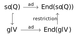
which suggests that we find the weight/eigenspaces for the $\mathfrak{so}(Q)$ action on $\operatorname{\mathfrak{gl}}V$, and then we intersect these spaces with the invariant subspace $\mathfrak{so}(Q)\leq \operatorname{\mathfrak{gl}}V$.

From our work on $\operatorname{\mathfrak{sl}}V$, we know how elementary diagonal matrices act on $\operatorname{\mathfrak{gl}}V$, i.e., we know that the $E_{i,j}$ were eigenvectors for the diagonal action, so these will be eigenvectors for the restricted diagonal action. To phrase things in our current notation for $\mathfrak{h}$ and $\mathfrak{h}^*$, we compute that the operator $\mathrm{ad}(\sum a_k H_k)$ on $\operatorname{\mathfrak{gl}}V$ sends \[\begin{aligned} E_{i,j} &\mapsto (a_i - a_j) E_{i,j}\\ E_{i,n+j} &\mapsto (a_i + a_j)E_{i,n+j}\\ E_{n+j,i} &\mapsto (-a_i - a_j)E_{n+j,i}\\ E_{n+j,n+i} &\mapsto (a_i - a_j)E_{n+i,n+j}, \end{aligned}\] for $1\leq j\leq n$. These span $V$ for the $m$ even case, otherwise we also should check \[\begin{aligned} E_{i,2n+1} &\mapsto a_i E_{i,2n+1}\\ E_{n+i,2n+1} &\mapsto -a_i E_{n+i,2n+1}\\ E_{2n+1,i} &\mapsto -a_i E_{2n+1,i}\\ E_{2n+1,n+i} &\mapsto a_i E_{2n+1,n+i} \end{aligned}\] to get a basis of $\operatorname{\mathfrak{gl}}V$ consisting of eigenvectors for the $\mathfrak{h}$ action. So, this gives us a decomposition of $\operatorname{\mathfrak{gl}}V$ as a sum of eigenspaces for the $\mathfrak{h}$ action, with

$L_i-L_j$ eigenspace spanned by $E_{i,j},E_{n+j,n+i}$
$L_i+L_j$ eigenspace spanned by $E_{i,n+j}$
$-L_i-L_j$ eigenspace spanned by $E_{n+i,i}$

and if $m$ is odd

$L_i$ eigenspace spanned by $E_{i,2n+1}, E_{2n+1,n+i}$
$-L_i$ eigenspace spanned by $E_{n+i,2n+1},E_{2n+1,i}$.

Now, we really wanted to study the action of $\mathfrak{h}$ on the smaller Lie algebra $\mathfrak{so}(Q)$, so we just intersect the eigenspaces with $\mathfrak{so}(Q)$ and find generators. We give them the following names. \[\begin{aligned} X_{ij} &= E_{i,j}-E_{n+j,n+i} \qquad \text{spanning $\mathfrak{g}_{L_i-L_j}$}\\ Y_{ij} &= E_{i,n+j}-E_{j,n+i} \qquad \text{spanning $\mathfrak{g}_{L_i+L_j}$}\\ Z_{ij} &= E_{n+i,j}-E_{n+j,i} \qquad \text{spanning $\mathfrak{g}_{-L_i-L_j}$}\\ U_i &= E_{i,2n+1} - E_{2n+1,n+i} \qquad \text{spanning $\mathfrak{g}_{L_i}$}\\ V_i &= E_{n+i,2n+1} - E_{2n+1,i} \qquad \text{spanning $\mathfrak{g}_{-L_i}$}. \end{aligned}\] Now, as $i\neq j$ range from $1,\dots,n$, together with $\mathfrak{h}$ we span $\mathfrak{so}(Q)$. So, this gives us the root space decomposition. We were in some sense lucky here—a-priori it could have happened that intersecting the weight spaces $\operatorname{\mathfrak{gl}}V$ with $\mathfrak{so}Q$, they drop too much in dimension and $\mathfrak{so}Q$ is not spanned by the intersections (e.g., think of $\mathbb{R}^2 = \mathbb{R}e_1 \oplus \mathbb{R}e_2$, but the subspace $\mathbb{R}(e_1+e_2) \leq \mathbb{R}^2$ meets $\mathbb{R}e_1, \mathbb{R}e_2$ at $0$, so not spanned by intersections). So, it was important for us to check that the intersections actually span $\mathfrak{so}Q$.

Next, following the representation theory program, we find the many representations of $\operatorname{\mathfrak{sl}}_2 \mathbb{C}$. Going through each type of root $\alpha$, we will write \[\mathfrak{s}_\alpha = \left\langle X_\alpha, Y_\alpha, H_\alpha\right\rangle\] for $X_\alpha,Y_\alpha$ generators of $\mathfrak{g}_\alpha$, $\mathfrak{g}_{-\alpha}$ respectively, and $H_\alpha \in [\mathfrak{g}_\alpha,\mathfrak{g}_{-\alpha}]$ (the coroot!) such that $\mathrm{ad}H_{\alpha}$ acts by $\pm 2$. Going through, one can check \[\begin{aligned} \mathfrak{s}_{L_i-L_j} &= \left\langle X_{ij},X_{ji},H_i-H_j\right\rangle\\ \mathfrak{s}_{L_i+L_j} &= \left\langle Y_{ij},Z_{ij},H_i+H_j\right\rangle\\ \mathfrak{s}_{L_i} &= \left\langle U_i,V_i,2H_i\right\rangle, \end{aligned}\] so the coroots are \[\begin{aligned} H_{L_i-L_j} &= H_i-H_j\\ H_{L_i+L_j} &= H_i + H_j\\ H_{L_i} &= 2H_i. \quad \text{for } \mathfrak{so}_{2n+1}\mathbb{C} \end{aligned}\] Now, we can find the weight lattice (with the root lattice inside). One can check that \[\Lambda_W = \left\langle L_1,\dots,L_n\right\rangle + \left\langle\frac{1}{2}\sum_i L_i\right\rangle\] (easy enough to see that these generators are all in $\Lambda_W$, and in general a functional $\sum a_i L_i$ is in $\Lambda_W$ when all $a_i-a_j$, $a_i+a_j$, and $2a_i$ are integral. It’s some sort of integer programming problem to see all of these are generated by our list.)

Now, we pick an ordering and describe the positive roots/Weyl chambers. Choose a linear form $\ell: \mathfrak{h}^* \to \mathbb{R}$ by sending $L_i \mapsto c_i$, where $c_1>c_2>\cdots>c_n>0$. Then, the positive roots of $\mathfrak{so}_{2n+1}\mathbb{C}$ are \[R^+ = \{L_i + L_j\}_{i<j} \cup \{L_i - L_j\}_{i<j} \cup \{L_i\}_i\] and for $\mathfrak{so}_{2n}\mathbb{C}$ we just also exclude the $\{L_i\}_{i}$.

The primitive positive roots are then \[\begin{aligned} &L_1-L_2,L_2-L_3,\dots,L_{n-1}-L_n,L_n \qquad\qquad \text{for $\mathfrak{so}_{2n+1}\mathbb{C}$}\\ &L_1-L_2,L_2-L_3,\dots,L_{n-1}-L_n,L_{n-1}+L_n \qquad \text{for $\mathfrak{so}_{2n}\mathbb{C}$}. \end{aligned}\]

Next, the Weyl chamber for $\mathfrak{so}_{2n+1} \mathbb{C}$ is given by \[\mathfrak{W}= \{\sum a_i L_i: a_1\geq a_2 \geq \cdots \geq a_n \geq 0\}\] since for $\alpha=\sum a_i L_i$, $\alpha(H_{L_k-L_{k+1}}) \geq 0$ will force $a_k\geq a_{k+1}$ and $\alpha(L_n)\geq 0$ forces $a_n\geq 0$.

The story for $\mathfrak{so}_{2n} \mathbb{C}$ is more complicated, since we do not have the positive root $L_n$ to pair against. Our next best thing are the primitive positive roots $L_{n-1} \pm L_n$, where the relation $\alpha(L_{n-1} \pm L_n)\geq 0$ implies \[a_{n-1}\geq |a_n|,\] giving us the Weyl chamber \[\mathfrak{W}= \{\sum a_i L_i: a_1\geq a_2 \geq \cdots \geq a_{n-1} \geq |a_n|\}.\]

Low Dimensional Examples

Proposition. $\mathfrak{so}_3 \mathbb{C}= \operatorname{\mathfrak{sl}}_2 \mathbb{C}$

Proof. We give a geometric proof. First, we have a short exact sequence \[0\to \left\langle\mu_3\right\rangle \to \mathrm{SO}_3 \mathbb{C}\to \mathrm{PSO}_3 \mathbb{C}\to 0,\] since the center of $\mathrm{SO}_3 \mathbb{C}$ are the matrices $\lambda I$ with determinant $1$, so $\lambda$ has to be a third root of unity.

So, $\mathrm{SO}_3 \mathbb{C}$ is a covering group of $\mathrm{PSO}_3 \mathbb{C}$, so they have the same Lie algebra.

Next, we can identify $\mathrm{PSO}_3 \mathbb{C}$ as a subgroup of $\mathrm{PGL}_3 \mathbb{C}$, since under the inclusion $\mathrm{SO}_3 \mathbb{C}\hookrightarrow \mathrm{GL}_3 \mathbb{C}$, the preimage of the center is the center. Then, we claim that \[\mathrm{PSO}_3 \mathbb{C}\hookrightarrow \mathrm{PGL}_3 \mathbb{C}\cong \mathrm{Aut}(\mathbb{P}^2)\] are exactly the automorphisms sending the conic $C=V(Q)$ back to itself, where $Q$ is the nondegenerate quadratric form in the definition of $\mathrm{SO}_3 \mathbb{C}$.

Let’s give the name $\mathrm{Aut}(\mathbb{P}^2,C)$ to the automorphisms $\phi$ of $\mathbb{P}^2$ with $\mathrm{im}\phi|_C \subseteq C$. So, our claim is \[\mathrm{PSO}_3 \mathbb{C}= \mathrm{Aut}(\mathbb{P}^2,C)\] as subsets of $\mathrm{PGL}_3 \mathbb{C}$. In proving this, we will review the identification $\mathrm{Aut}(\mathbb{P}^2) \cong \mathrm{PGL}_3 \mathbb{C}$.

First, we describe how to turn an element $[A]\in \mathrm{PSO}_3 \mathbb{C}$ into an automorphism. First, pick a representative $A$ of the equivalence class, which is an element of $\mathrm{GL}(V)$, where $V=\mathbb{C}^3$. Then, take the pullback to get $A^* \in V^*$. Next, apply the $\mathrm{Sym}^\bullet$ functor, i.e., if we identify \[S = \mathrm{Sym}^\bullet V^* \cong \mathbb{C}[x,y,z],\] we define \[f_A = \mathrm{Sym}^\bullet A^*: S\to S\] by sending $ax+by+cz$ to the image of the (column) vector $(a,b,c)$ under $A^*$ (the transpose).

Then, because $A^*$ is surjective, when we apply the $\mathrm{Proj}$ construction, we get an everywhere-defined morphism \[\phi_A: \mathbb{P}^2 \to \mathbb{P}^2.\]

Now, we want to check that \[\mathrm{im}\phi_A|_C = C.\] Essentially, this is just the following: identify a closed point $P\in \mathbb{P}^2$ with a line $\ell\in V$, and then $Q(\ell)=0$ iff $Q(A\ell)=0$ by assumption.

The only complications are to check that $\phi_A$ indeed acts on closed points in this fashion (which is standard), and that $\phi_A$ sends the generic point of $C$ to $C$ ( argue by closure/specialization?).

So, indeed $\phi_A$ is in $\mathrm{Aut}(\mathbb{P}^2,C)$.

Conversely, let $\phi\in \mathrm{Aut}(\mathbb{P}^2,C)$. In the proof of $\mathrm{Aut}(\mathbb{P}^2)=\mathrm{PGL}_3(\mathbb{C})$, we get that \[\phi = \phi_A = \mathrm{Proj}\mathrm{Sym}^\bullet A^*.\] We want to show that assuming $\phi_A(C) = C$, that $[A] \in \mathrm{PSO}_3(\mathbb{C})$, which is to say that $A\mathbb{C}^* \cap \mathrm{SO}_3 \mathbb{C}$ is nonempty. By replacing $A$ with $\frac{1}{\sqrt[3]{\det A}} A$, the problem becomes showing $A\in \mathrm{SO}_3 \mathbb{C}$ on the nose.

From $\phi(C) = C$, we at least get the following. Let $\ell\leq \mathbb{C}^3$ a line representing a closed point in $\mathbb{P}^2$. Then, we know $Q(\ell)=0$ iff $Q(A\ell)=0$.

Now, we want to deduce $A$ preserves $Q$ from these facts/assumptions. Here, we cite the classical projective Nullstellensatz. We’ve gotten \[V_p(QA)=C=V_p(Q),\] so $\sqrt{(QA)} = \sqrt{(Q)}$, so $QA = \lambda Q$, and by our assumption that $\det A=1$, we get $\lambda = 1$, so $QA=Q$.

So, we’ve succeeded and $\mathrm{Aut}(\mathbb{P}^2,C)=\mathrm{PSO_3}(\mathbb{C})$.

Next, we claim $\mathrm{Aut}(\mathbb{P}^2,C) \cong \mathrm{Aut}(C)$ by showing every automorphism of $C$ lifts to a unique automorphism of $\mathbb{P}^2$. We can take $C$ to be the degree 2 rational normal curve (the Veronese embedding of $\mathbb{P}^1$).

We claim that the following is an extension of the $C$ automorphisms to $\mathbb{P}^2$. We have $\mathrm{GL}_2 \mathbb{C}$ acting not just on $\mathbb{C}^2$ (the cone over $\mathbb{P}^1$), but on $\mathrm{Sym}^2 \mathbb{C}^2\cong \mathbb{C}^2$ (the cone over $\mathbb{P}^2$), and then we can descend to the projective general linear groups.

This gives us a map $\mathrm{Aut}(\mathbb{P}^1)\cong\mathrm{Aut}(C) \to \mathrm{Aut}(\mathbb{P}^2)$ extending the automorphisms. We argue that these extensions are unique by showing that for any other morphism, we can postcompose it by something in $\mathrm{Aut}(C)$ until it is identity on $C$, and then arguing that any automorphism of $\mathbb{P}^2$ that fixes $C$ must be identity.

To see this, first note that the fixed points of an automorphism of $\mathbb{P}^2$ is a union of linear subspace, since for $\phi_A$ a line $\ell=\left\langle v\right\rangle$ is fixed exactly when $Av=\lambda v$, so the fixed points are the lines inside \[\bigcup_{\lambda\in \mathbb{C}^*} \ker(A-\lambda I),\] (where the kernels are nonzero for finitely many $\lambda$ because these are eigenvalues of a finite dimensional operator). So, if $C$ is fixed, then $C$ is inside a union of linear subspaces, and by irreducibility, it must be a line, but this contradicts it being degree 2.

Thus, we see that $\mathrm{Aut}(\mathbb{P}^2,C)\cong \mathrm{Aut}(C)$, which is just $\mathrm{PGL}_2(\mathbb{C})$.

Finally, we argue that the composition \[\mathrm{SL}_2 \mathbb{C}\to \mathrm{GL}_2 \mathbb{C}\to \mathrm{PGL}_2 \mathbb{C}\] is a covering map. This is maybe not a very geometric argument, but one could see this by seeing the differential is an isomorphism at the identity. ◻